

Identifying the S arrival on AS-1
Seismograms and
estimating distance using the S minus P
method 1
|
|
Larry BraileProfessor,
http://web.ics.purdue.edu/~braile/ February, 2008 |

Introduction: Recognizing the S wave (direct S arrival) on a seismogram is very useful as it often can be used to make a good estimate of the epicenter-to-station distance using the S minus P method. Identifying the S arrival on seismograms recorded by the AS-1 seismograph (or any other seismograph that records only the vertical component) can be difficult or impossible due to the insensitivity of the seismometer to horizontal ground motions. The direct S arrival is often present in the distance range of zero to 105 degrees (distance measured in degrees geocentric angle; one degree is equivalent to 111.19 km along the surface) from the epicenter. An example of an AS-1 seismogram displaying a clear S arrival is provided in Figure 1. At distances of 105 to as much as 140 degrees from the epicenter, both the direct P and direct S arrivals are diffracted by the core and may still be visible and used in the S minus P method.
This document is available for viewing with a browser (html file) and for downloading as an MS Word document or PDF file at the following locations:
http://web.ics.purdue.edu/~braile/edumod/as1lessons/Swave/Swave.htm
http://web.ics.purdue.edu/~braile/edumod/as1lessons/Swave/Swave.doc
http://web.ics.purdue.edu/~braile/edumod/as1lessons/Swave/Swave.pdf
[1]  Last
modified September 15, 2008
Last
modified September 15, 2008
The web page for
this document is:
http://web.ics.purdue.edu/~braile/edumod/as1lessons/Swave/Swave.htm
Partial funding for this development provided by the National Science Foundation.
ã Copyright 2008. L. Braile. Permission granted for reproduction for non-commercial uses.
The travel times of P and S arrivals, along with other phases, are shown in the standard travel time curves in Figure 2. Note that as the epicenter-to-station distance increases, the S minus P travel time also increases. This relationship allows epicenter-to-station distance estimation from the S minus P time from a single seismogram. Because many earthquakes occur at distances greater than 105 or 140 degrees from a single station, the method cannot be used for all recorded events. Additionally, because the AS-1 is a vertical component seismograph, the S wave is not always recognizable. In practice, it is possible to identify the direct S arrival and use the S minus P method on about one third of all events recorded by the AS-1 seismograph. In these cases, the epicenter-to-station distance can be determined with reasonable accuracy (Figure 3). The epicenter-to-station distance and theoretical travel times can be calculated from the epicenter and station coordinates (latitudes and longitudes) using the USGS travel time calculator website at: http://neic.usgs.gov/neis/travel_times/.
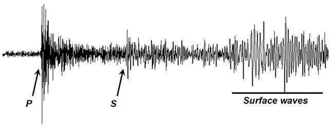
Figure 1. Seismogram recorded by
the AS-1 seismograph. S wave (“direct” S
arrival) is identified by approximate time position in the seismogram, large
relative amplitude, and lower frequency than the preceding P arrivals.
Suggested procedure for S arrival identification: The following procedure is suggested to recognize the direct S arrival on AS-1 seismograms and estimate the distance using the S minus P method. If the epicenter is known to be greater than about 140 degrees from the station, the direct S arrival will not be present. If the epicenter is between 105 to 140 degrees distance from the station, the first arriving P and S arrivals will be diffracted by the core and are often of small amplitude or not recognizable, particularly for distances greater than about 110 degrees.
1. A rough epicenter-to-station distance estimate (local [<5 deg.], regional [5 to 20 deg.], distant [20 to 90 deg], very distant [>90 deg.] – distant and very distant are often called “teleseismic”) can be determined by comparison of the signal duration (in general, the duration is greater for greater distance) and character of your seismogram with the seismograms in the InterpSeis catalog of events available online at:
http://web.ics.purdue.edu/~braile/edumod/as1lessons/InterpSeis/InterpSeis.htm. Another rough estimate of epicenter-to-station distance can be made using the Surface wave minus P wave times. Find the ~20 s period surface wave arrival (usually the largest surface wave amplitude) time and the first arriving P wave time. Measure the difference between these times in minutes. The approximate distance in degrees will be about 2 times the time difference (Figure 4). This method only works for seismograms that have prominent surface waves and for distances that are great enough (usually about 50 degrees or greater) such that the 20 s period surface waves are visible. Knowledge of the approximate epicenter-to-station distance can be useful in recognizing or refining your S-wave arrival time.
Figure 2. Standard travel time curves for surface focus
events.
Figure 3. Comparison of distance
estimated by the S minus P method for AS-1 seismograms with the calculated
distance from the USGS epicenter location.
Figure 4. Example of approximate
epicenter-to-station distance calculation using the difference in time between
the P and surface wave arrivals. Actual
distance is 25.96o.
2. The S wave (if visible) is located on the seismogram a little less than half way from the P wave to the surface wave. Surface waves will not be prominent or visible for deep focus earthquakes. The S arrival is also often characterized by large amplitude and a frequency change (from high frequencies associated with P wave energy to lower frequencies). This frequency change can be seen by the separation of lines in the S arrival shown in Figure 1. One can better view and analyze the frequency change by zooming in on the arrival using the AmaSeis seismogram extraction tool.
3. The S wave can often be enhanced by filtering
the seismogram. For distant events, try
a
4. To view the P and S wave and use the AmaSeis travel time tool to estimate the epicenter-to-station distance, extract (select with the cursor) the seismogram from about 5 minutes before the P wave through the first few peaks of the surface waves. Filter the seismogram if needed, and pick the P and S arrivals with the AmaSeis arrival time pick tool. Select the travel time tool to view the seismogram on the standard travel time curves. Because the AmaSeis software automatically selects the distance range shown on the travel time curve display from the length of the seismogram, it may be desirable to select (extract) only a portion of the seismogram (or re-open the full record if you have extracted only a short segment of the seismogram) in order to obtain the desired travel time curve display and accurately align the P and S arrivals on the travel time lines. Move the seismogram with the cursor until the P and S arrival times match the curves. Additional information on the AmaSeis tools and the S minus P method can be found in the Using AmaSeis tutorial at:
http://web.ics.purdue.edu/~braile/edumod/as1lessons/UsingAmaSeis/UsingAmaSeis.htm.
Sample seismograms for identification to the S arrival and estimation of distance using the S minus P method: Sample seismograms (from the WLIN AS-1 station catalog) for practice in picking the S arrival time are listed in Table 1. Links to the twenty WLIN sac file seismograms are contained in Table 2. Download the seismograms to the sac folder in your AmaSeis folder. The seismograms can then be opened, viewed, filtered and analyzed using the AmaSeis software.
Table 1. WLIN seismograms for S
arrival identification and estimation of epicenter-to-station distance using
the S minus P method. (Additional information on the earthquakes corresponding
to these seismograms can be found in the WLIN earthquake catalog at: http://web.ics.purdue.edu/~braile/edumod/as1lessons/InterpSeis/EqList.xls)
|
Date (yymmdd) |
Approx. Time
(hh:mm) |
“Difficulty” (1
= easiest) |
Distance
from S –
P time (deg.) |
Comments |
|
|
1 |
00/06/02 |
11:20 |
1 |
|
|
|
2 |
02/12/23 |
13:52 |
1 |
|
|
|
3 |
04/09/09 |
16:38 |
1 |
|
|
|
4 |
04/11/15 |
09:14 |
1 |
|
|
|
5 |
04/11/12 |
06:46 |
1 |
|
|
|
6 |
05/06/13 |
22:54 |
1 |
|
|
|
7 |
06/10/15 |
17:18 |
1 |
|
|
|
8 |
08/02/21 |
14:21 |
1 |
|
|
|
9 |
00/05/12 |
18:54 |
2 |
|
|
|
10 |
00/08/09 |
11:47 |
2 |
|
|
|
11 |
01/01/26 |
03:05 |
2 |
|
|
|
12 |
03/02/19 |
03:42 |
2 |
|
|
|
13 |
03/05/14 |
06:10 |
2 |
|
|
|
14 |
03/12/22 |
19:22 |
2 |
|
|
|
15 |
03/12/25 |
07:18 |
2 |
|
|
|
16 |
04/06/10 |
15:30 |
2 |
|
|
|
17 |
05/06/17 |
06:28 |
2 |
|
|
|
18 |
05/07/13 |
12:15 |
2 |
|
|
|
19 |
05/06/15 |
02:57 |
3 |
|
|
|
20 |
06/05/24 |
04:26 |
3 |
|
|
Table 2. WLIN S-wave seismogram links.