EQlocation

The AS-1 Seismograph – Installation and Calibration ¹

L. Braile, November, 2002;

Updated November 2004

http://web.ics.purdue.edu/~braile

Introduction: The AS-1 Seismometer (http://www.amateurseismologist.com/, http://jclahr.com/science/psn/as1/) and the data acquisition software AmaSeis (http://www.geol.binghamton.edu/faculty/jones/), written by Dr. Alan Jones, SUNY, Binghamton), form an easy-to-use and effective seismograph for educational purposes. Earthquake data can be recorded, analyzed and archived using the AS-1 and a computer running Windows. The seismometer (Figure 1) is inexpensive (less than $500), utilizes a simple design so that the principles of a seismometer and the recording of ground motions can be understood, and, with the AmaSeis software, provides for efficient monitoring of earthquakes through recording and display of continuous seismic data. The software allows easy selection and display of portions of the seismic data so that seismograms corresponding to specific earthquakes or other signals can be enlarged, filtered, viewed on the screen and saved for further use or additional analysis. Seismograms displays can also be printed. Arrival times of prominent phases, such as P and S waves, can be identified on the extracted seismograms and compared with standard travel time curves so that the distance earthquake epicenter to the recording location can be determined. The operation of the AS-1 with the AmaSeis software is described in tutorial and help files supplied with the software. Furthermore, using the procedures described here, magnitude estimates of earthquakes recorded on the AS-1 seismograph can be calculated from relatively simple equations and information read from the seismic data. The suggestions provided here result from experiences with operating an AS-1 seismograph for nearly 5 years (four and one half years with the AmaSeis software) in West Lafayette, Indiana. The seismograph is located on a cement slab floor in the basement of a house. Earthquakes that generated seismograms that are of sufficient signal strength to use for estimating the magnitude of the event occurred, on the average, about once a week. Recognizable signals from distant earthquakes were recorded at about twice that rate. Twelve regional (within about 1500 km from the seismograph) events were recorded since January 1, 2000.

[1] Last modified November 21, 2004

The web page for this document is:

http://web.ics.purdue.edu/~braile/edumod/as1mag/as1mag1.htm.

Partial support for this development provided by IRIS and the National Science Foundation.

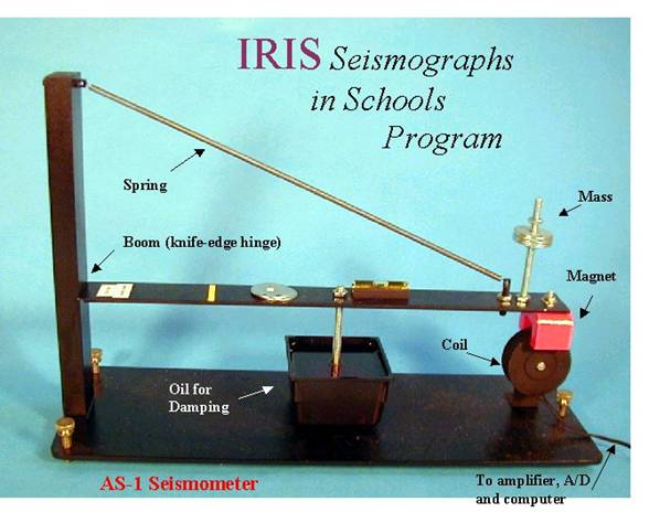
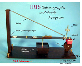
Figure 1. The AS-1 seismometer showing the main components of the instrument. The AS-1 is a vertical component seismometer. Up and down motions of the ground, and therefore of the base and frame of the seismometer, cause the coil to move relative to the magnet that is suspended by the spring and boom assembly. The mass of the seismometer, consisting primarily of the magnet, boom and the washers, tends to remain steady because of inertia when the base moves. The motion of the coil relative to the magnet generates a small current in the coil. The current is amplified and digitized by an amplifier unit (not shown) and connected to the computer for recording and display. The damping (using oil in the container and a washer mounted to a bolt extending downward from the boom into the oil) reduces the tendency for the mass and spring system to oscillate for long duration from a single source of ground motion (arrival of seismic waves at the location).

Example Seismograms: When a very large earthquake occurs anywhere in the world (or a smaller event that is located closer to the seismograph station), the AS-1 seismometer responds to the small ground vibrations that are generated by the earthquake and propagate from the earthquake location to the seismograph station. The ground vibration is converted by the seismometer to a small electrical current that is converted to a digital signal that is sent to an attached computer and the AmaSeis software. An example of a recorded earthquake is shown in Figure 2. This record is from a very large event located about 42 degrees (4670 km) away from the AS-1 seismograph in West Lafayette, Indiana.

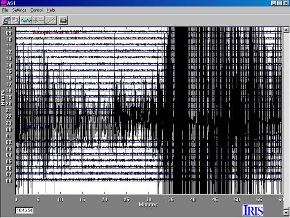
Figure 2. Screen image of 24-hour AS-1/AmaSeis record for November 3-4, 2002 showing the magnitude 7.9 central Alaska earthquake. Seismograph gain was 60. First arrival is at about 22 hours and 21 minutes (UTC/GMT or about 5:21 PM local, EST time). Seismogram recorded at West Lafayette, Indiana. Every year, about 1-2 earthquakes of this magnitude or larger occur somewhere in the world (http://neic.usgs.gov/neis/eqlists/eqstats.html).

A close-up view of the November 3, 2002 seismogram recorded by the AS-1 seismograph at West Lafayette, Indiana is given in Figure 3. Because some of the surface wave arrivals were so large, part of the recording is “clipped.” This signal distortion is caused by the inability of the digitizer in the electronic circuitry of the seismograph to properly convert the largest electrical signals (in this case resulting from ground vibrations of greater than about 1 mm of ground displacement at the seismograph station) to digital values. When ground vibration shakes the seismometer, a small electrical current is generated in the seismometer’s coil. This signal is amplified and the resulting signal converted to digital numbers that can be recorded by the AmaSeis software. The digitizer is capable of producing digital signals in the range of -2048 to +2048 (integers; the digitizer actually produces values of 0 – 4096, but the average value, 2048, is subtracted from the result). When electrical signals that should be converted to digital values that are larger than +2048 or smaller than -2048 are produced, the digitizer can only produce the extreme values (-2048 or +2048) resulting in the truncation or clipping that is seen on the seismogram in Figure 3.

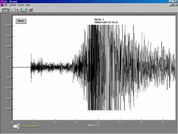
Figure 3. Close-up of November 3, 2002 central Alaska earthquake record from West Lafayette, Indiana (extracted from the 24-hour record, Figure2, using seismogram extraction tool in AmaSeis). Note that the amplitudes of the surface wave arrivals from about 14 to 24 minutes after the first arrival are “clipped” (cut off by the digitizer in the AS-1 seismograph because the amplitudes are larger than can be converted properly by the electronic circuits).

Although the AS-1 seismograph is a relatively simple and inexpensive seismograph, it is capable of relatively accurate and effective recording of ground vibration from earthquakes and other sources. A comparison between an AS-1 seismogram for the November 3, 2002 earthquake and a seismogram recorded by a modern, high-performance (and much more expensive) seismograph is shown in Figure 4. Although the seismograms differ in detail (the instruments have different responses and were locate about 5 km apart on somewhat different near-surface materials), the main features and distinct arrivals are very similar. However, modern, high-performance seismographs that are used by seismologists for research and earthquake monitoring have very accurate timing and calibration, very low electronic noise, and are capable of recording a broader range of ground vibration amplitudes and signal frequency range. Also, research seismographs usually record three components of ground motion (vertical and two horizontal directions) rather than just the vertical component as in the AS-1 seismograph.

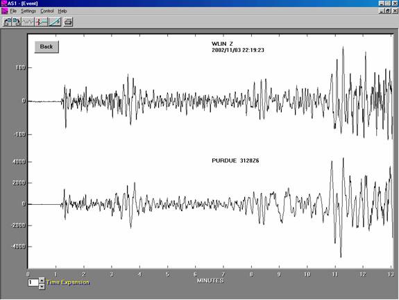
Figure 4. Comparison of the first 12 minutes of the November 3, 2002 central Alaska earthquake seismogram (upper trace; band pass filtered from 0.001 – 0.1 Hz in AmaSeis) recorded by an AS-1 seismograph at West Lafayette, Indiana with a similar seismogram (lower trace; band pass filtered from 0.1 – 2 Hz in AmaSeis) recorded by a Guralp high-performance, broadband, digital seismograph at West Lafayette, Indiana. Both seismograms are vertical component records. The seismograph stations are about 5 km apart.

To see an online AS-1 record from Boston College (Prof. Alan Kafka) that is updated every 10 minutes, go to:

http://www2.bc.edu/~kafka/Seismograph_Display/EarthMoves.html. For more information on this online seismograph display, see

http://www2.bc.edu/~kafka/AS1_Web_Tool/Seismo_Display.html. This site also includes links to some sample recordings of earthquakes at the Boston College AS-1 seismograph stations. The WLIN near-real time seismograph display can be viewed at:

http://web.ics.purdue.edu/~braile/AS1Display/AS1display.jpg.

Notes on Installing the AS-1 Seismograph and the AmaSeis Software:

Installing the AS-1 Seismometer:

Assemble the AS-1 seismometer as described in the instructions provided with the seismometer. More detailed instructions are also available in the manual at http://www.scieds.com/spinet/AS1AmaSeis_v2.pdf. The seismometer will work best in a quiet environment. The most important factor is placing it on a solid floor – concrete slab basement or first level is best. However, the seismometer will work nearly anywhere at lower gain setting, including on an upper level floor of the building and on a table top (for testing and demonstration). Because the instrument is not very sensitive to high frequency signals, vibrations from walking near the seismometer are small unless one is walking within a couple of meters of the seismometer. For this reason, it is desirable to place the connected computer and display at least 2 meters away from the seismometer.

Be sure to level the base with the leveling screws and the boom by moving the level bubble and a washer along the top surface of the boom until the boom is approximately level. This process, and the addition of masses (washers on the bolt at the end of the boom), must be repeated when oil (use 10W40 motor oil) is added to the container and the washer extending downwards from the boom is positioned in the oil for damping. Place a drop of the motor oil on the hinge of the boom (be very careful of the sharp edge and do not damage the edge) to help prevent friction on the hinge. Be sure that the magnet and coil assemblies are positioned as shown in the instructions and that the magnet and coil do not touch when the boom (and magnet) are moved up and down. When you are ready to connect to the computer and set up the software (see below; we suggest that you do not use the software provided with the AS-1 seismometer, use the AmaSeis software instead, http://www.geol.binghamton.edu/faculty/jones/), carefully place the clear plastic cover over the seismometer to decrease air currents on the spring which cause significant noise.

To test the instrument, be sure that the output is approximately “centered” (see below), walk up close, or jump near to the seismometer and you should see a small noise pulse on the screen. Gain levels for reasonably quiet sites (concrete slab or floor installation) should be about 20 to 60. See 24 hour seismogram record, Figure 5, below for example of relatively small noise level. At this level, one should record the following events (sometimes the signal will be visible but no distinct arrivals will be distinguished and amplitudes will be so small that measuring amplitudes for magnitude calculation will be impossible; sometimes very clear arrivals and amplitude will be visible):

Local earthquakes (0 – 5 degrees distance) – magnitude ~3.5+

Regional earthquakes (5 – 20 degrees distance) – magnitude ~4.5+

Distant earthquakes (20 – 90 degrees distance) – magnitude ~6.0+

Very distant earthquakes (90 – 180 degrees distance) – magnitude ~6.5+

(these “rules of thumb” will depend on the site and gain level, your location, for example, western US or eastern US, and the nature of the earthquake and the path that the waves have traveled from the earthquake location to your station).

My experience is that a very “visible” earthquake signal is recorded, on the average, of about once a week. About half of these can be used to calculate a magnitude (mb or MS) and about a fourth are at distances of less than 105 degrees and have S arrivals that are distinct enough (usually after filtering with a 0.001 to 0.2 Hz bandpass filter in AmaSeis; the S arrival is often best seen by the lower frequency arrival) to pick an S-P time (using the arrival picking tool in AmaSeis) and estimate the distance to the event using the S-P and travel time curve matching tool in AmaSeis.

Setting up the AmaSeis software:

1. Help file for AmaSeis:

AmaSeis (http://www.geol.binghamton.edu/faculty/jones/), has a fairly complete help file that includes instructions for setting up the software, options that are available for analyzing and displaying data, and a tutorial. To obtain help information, click on the Help icon (menu) at the top of the screen, and then on Help topics. Select Contents. Double-click on one of the topics and then on one of the question marks that appears before the name of a sub-topic, then use the double-arrow controls (right or left arrows at the top of the Help dialog box) to find information related to that topic. To investigate a specific topic, feature or setting, select Index from the Help topics dialog box, and double-click on the appropriate entry. An online tutorial with detailed descriptions for the use of the AmaSeis software is also available at:

http://web.ics.purdue.edu/~braile/edumod/as1lessons/UsingAmaSeis/UsingAmaSeis.htm.

2. Settings For AmaSeis:

Settings Menu

Helicorder

Lines per hour: usually set to 1 (gives a 24 hour record on screen which is useful for monitoring because when you observe the screen once per day, you will know immediately if an earthquake has occurred; to go back to look at earlier data, use the scroll bar on the right); can be set to as high as 20 (60 in the latest release of AmaSeis) so that the cursor moves quickly across the screen and the details of the waveform can be seen; this setting is useful for laboratory testing and demonstrations and “make your own earthquake” (stomp test, etc.) activities; for lines per hour greater than 1, temporarily set the decimate factor to 1.

Gain: amplification of the signal by the software; set to 1 for set up and initial centering of the trace on the screen, then to a higher number depending on the noise level; in reasonably quiet installations, a gain of 50 or more is possible.

Low pass filter cutoff: low pass filter option for the trace on the helicorder screen display; set at 3 Hz; if high frequency noise is visible on the screen, try a lower cutoff such as 1 or 0.5Hz to see if the noise is reduced; earthquake signals will generally not be greatly affected by this cutoff frequency for this seismometer.

Days to retain record: this value controls how far back in time one can scroll (if you are scrolling back more than a few days, move the scroll bar slider with the mouse instead of using the up or down arrows or clicking on the bar above or below the slider) to view the seismic data on the screen; set to 365 to allow viewing data back as far as one year; the value can be set larger, but if there are old data that you would like to view, they usually would have been saved as individual events (extracted and saved as .sac files; so that data archive doesn’t get too large) and then opened under the File menu.

Decimate factor: Set to 10, normally; this setting will provide a fairly accurate view of the data on the screen but allow rapid scrolling; a decimate factor of 10 plots only every 10^th point; some distortion is caused by this choice, so for large numbers of lines per hour, “make your own earthquake” experiments, and whenever you want to see the most accurate view of a seismogram on the screen, set the decimate factor to 1. The decimate factor does not affect the plotting of an extracted seismogram which is always plotted with all of the available points.

Settings

Show data values

This dialog box and display allows one to center the cursor so that it tracks approximately on the “zero line” (blue line) that is defined for each hour. To center the trace, it is convenient to start with a low gain setting (such as 1). Turn the black knob on the small black interface box that comes with the AS-1 seismometer that between the seismometer and the computer in the electric circuit. The knob adjusts the cursor position on the screen. It is very sensitive, so make small adjustments and determine which way to turn the knob in order to cause the cursor to move upwards. As you adjust the knob, the cursor should get closer to the zero line and the display numbers should be close to zero. When you have succeeded in getting the numbers close to zero, turn the gain up and repeat, eventually setting the gain to the highest level that is consistent with the background noise (you should see relatively continuous, small, about +/- 1 to 2 mm, movements on the screen), and making the displayed values close to zero. To adjust the knob when the gain is set to a high value (greater than about 10), it is convenient to use a pencil and very, very lightly tap the knob from the side to cause it to move. THIS CENTERING PROCESS CAN TAKE CONSIDERABLE TIME – PROCEED SYSTEMATICALLY AND PATIENTLY.

Archiving data:

Recording the AS-1 seismic data with the AmaSeis software generates about 1 MB of data per day. If you computer has insufficient disk space to archive data for many months or years, you can copy the files onto a zip disk or to a CDR. Alternatively, you can sort through the recorded data and delete data for days in which there was no significant signal. An example of a 24-hour record from the AS-1 seismometer and the AmaSeis software is shown in Figure 5.

Figure 5. Example of screen image. Gain setting at 60 (relatively quiet site in basement, on concrete slab). Note noise level. The event at about 7 hours and 10 minutes is a magnitude 6.7 earthquake near the north island of New Zealand. Prominent P wave arrivals and surface waves (longer period wave train) are visible. The light, straight lines are “zero lines” that mark the approximate location of the data for each hour of the day. The “wiggly lines” are the output of the seismometer and display both background “noise” and seismic signals generated by earthquakes or other identifiable sources. The noise level is fairly low for this record. Noise levels are typically a little higher during the winter months, during periods of high wind, and when large storms are located near the coast producing significant microseisms.

4. Time Synchronization and Maintaining a Seismograph Catalog:

It is useful and “good scientific practice” to develop a catalog for your seismograph station. Entries are made to the catalog every day or two that include absolute time checks or synchronizations (comparing the computer clock display to an accurate, absolute time signal such as from a radio-synchronized clock (arctime.com) or radio station WWV, 5, 10 or 15 MegaHertz frequency, on a short wave radio; alternatively, if the computer is connected to the internet, the computer clock can be periodically synchronized to absolute time using the software tool AboutTime, http://www.arachnoid.com/), times of arrivals (and amplitude and magnitude information) of earthquakes that are recorded by the seismograph, and comments about the weather or background noise conditions or operational status of the seismograph.

A very convenient radio synchronized clock (“Atomic Clock”) is the SkyScan wall or desk clock (I purchased one at our Sam’s Club store for $20; Figure 6) that has very large lettering. The clock can be set to show GMT time and can be used to visually check the time correction of your computer running AmaSeis and to record the “drift” of the computer clock. Occasionally resetting (“synchronizing”) the computer clock to GMT time will keep the AmaSeis time display reasonably accurate. A time correction can be applied to saved seismogram files in AmaSeis. The atomic clock makes a nice display for GMT time even if you have an Internet connection on your computer that is used to run AmaSeis and can update your computer clock automatically using the Internet tools described above. The SkyScan Atomic Clock is also available ($30) at: http://eggshop.net/skysatcloc.html, or, http://homestore3.com/skysatcloc.html. Another atomic clock option (with large digits display) is the WS-8001U wall clock from La Crosse Technology, available at: http://www.weathermeter.com/ ($40).

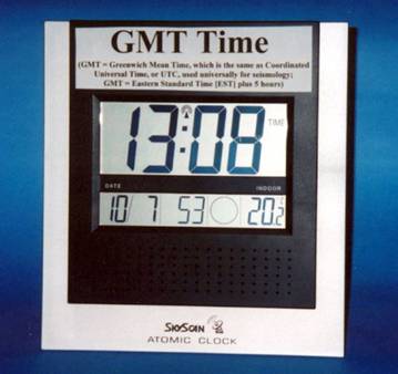
Figure 6. SkyScan atomic clock. A label describing GMT or UTC time was added.

Relative Calibration of the AS-1 Seismograph: A relative calibration of the AS-1 seismograph can be conducted using a “step function” method. A step function (a small, sudden increase or decrease in the position of the mass with respect to the coil) can be applied to the seismometer by lowering (or removing) a small mass onto the boom of the instrument. Because lowering the mass causes an inconsistent input to the seismometer, the method works best by lifting the mass. Because the seismometer is very sensitive, the relative calibration process, although simple, must be performed with a very specific procedure and very carefully. To perform the calibration, use a piece of masking tape or post-it note material to mark a position on the boom of the AS-1 seismometer that is 10 cm from the hinge and upright. Place the cover back over the instrument and drill a small hole (~4mm or 1/8 in) in the top of the cover above the mark on the boom. Make the mass used for calibration by cutting a 1 x 2 cm rectangle of lightweight poster board. This mass is about 0.063 g. Fold the poster board rectangle into the shape of a “tent” and attach a 3 m long piece of nylon monofilament thread (very light; available in fabric and sewing stores) to the top of the poster board tent with a small piece of tape. Thread the monofilament through the hole in the cover (from the inside of the cover) so that the small mass is suspended above the mark on the boom by the thread. Because the instrument is sensitive to tilt if one is standing near it, and because the air current noise is large, put the cover on, and lower the mass through the small hole in the top of the cover by holding the other end of the thread (it is convenient to attach a piece of tape to the free end of the thread to make it easier to find and hold on to the end of the thread) from a distance of about 3 m away, standing still. Lowering the mass gives a calibration pulse, but a better pulse (about 1400-1500 counts maximum amplitude) is obtained by letting the instrument stabilize and then pulling on the thread to lift the mass suddenly off the boom. This method appears to be stable and results in calibration pulses (Figure 7) that varied only about +/- 10% between tests. The maximum amplitude of this test should provide a relatively linear correction factor to the amplification of different instruments. For more information on calibration of the AS-1 seismometer, see http://quake.eas.gatech.edu/MagWeb/CalReptAS-1.htm.

This relative method of calibration has the following uses:

1. Performing the calibration tests to see if the seismometer is working properly (the calibration pulse should look approximately like the one in Figure 7; the “lifting the mass” pulse is used; the calibration pulse is extracted from the standard AmaSeis display to view it in a close-up view). Repeated calibrations suggest that measurable values of the calibration test pulse should be (approximately):

amplitude of first trough (negative) = -1420 +/- 150 counts

amplitude of first peak (positive) = 480 +/- 50 counts

time from beginning of calibration pulse to first zero crossing = 3.0 +/- 0.5 seconds

2. The relative calibration allows one to compare different instruments. AS-1 seismographs that have calibration pulses that are approximately the same as the pulse in Figure 7 can be assumed to have the same displacement amplification values as given here, and can be used to estimate magnitudes using the amplification values and procedures described here. If the calibration pulse for a different AS-1 seismometer is similar to the one shown in Figure 7 (and parameters given above) but has different maximum amplitude, one can adjust the amplification factors used in the magnitude calculations by the relative difference between the two AS-1 instruments.

3. The calibration provides a check on the polarity of the seismometer. Because lifting the mass from the boom causes the boom to move up relative to the coil that is attached to the base of the seismometer, the first motion of the output trace (the calibration pulse) should be down or negative. (A first “up” motion of the ground from an incoming seismic wave will move the base and the coil up relative to the magnet [corresponding to a relative down motion of the boom] attached to the boom, because of inertia of the seismometer mass suspended by the spring. This up motion of the ground will therefore cause an up or positive signal on the seismograph trace.) If the calibration pulse (corresponding to lifting the small mass) has a first positive motion, the polarity of the seismometer is reversed. To correct the polarity, simply switch the input wire connections on the AS-1 amplifier box.

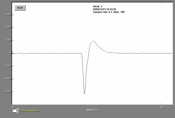
Figure 7. Calibration pulse created by suddenly lifting a small mass (0.063 g) from the boom (at a location 10 cm from the hinge) of the AS-1 seismometer. Enlarging (by selecting and extracting in the AmaSeis program) the calibration pulse allows one to measure the characteristic parameters of the pulse (maximum amplitude of the two peaks of the pulse and time between the start of the pulse and the first zero crossing) for comparison between instruments.

Additional information on installation and operation of an AS-1 seismograph is available at: http://www.scieds.com/spinet/AS1AmaSeis_v2.pdf (a complete manual for setting up the seismograph, using the AmaSeis software and interpreting the recorded seismic data).

Return to Braile’s Earth Science Education Activities page

The AS-1 Seismograph –Magnitude Determination