|
Feb. 27, 2010 M8.8 Chile Earthquake: Seismic/Eruption
Views, Seismicity, Main Shock-Aftershock Sequence L. Braile, May, 2010
|
|


1. Introduction: The February 27, 2010 M8.8 Chile earthquake was one of the largest earthquakes of the past few decades and occurred about 260 km north of the May 22, 1960 M9.5 Chile earthquake that is the largest known earthquake in history. The February 27 (3:34:14 am local time, 06:34:14 UTC), 2010 M8.8 Chile earthquake caused substantial damage and loss of life. There are also many interesting seismological and earthquake hazards aspects of this event. In this activity, we present some downloadable files that can be used with the Seismic/Eruption program to view and explore the earthquake history of the area, the February 27, 2010 M8.8 Chile earthquake and its associated aftershocks, the plate tectonic setting for earthquakes along the west coast of South America, and some examples of earthquake hazards and damage. The information presented here should be of interest for teachers, particularly those who already are familiar with the Seismic/Eruption program or would like to learn use it, and who would like to enhance their teaching of earthquakes and earthquake related topics. Detailed information about the February 27, 2010 M8.8 Chile earthquake can be found at the U. S. Geological Survey site at:
http://earthquake.usgs.gov/earthquakes/eqinthenews/2010/us2010tfan/.
[1]  Last modified May 28, 2010
The web page for
this document is:
http://web.ics.purdue.edu/~braile/edumod/chile/chile.htm
PDF version: http://web.ics.purdue.edu/~braile/edumod/chile/chile.pdf
Partial funding for this development provided by the National Science Foundation.
ã Copyright 2010. L. Braile. Permission granted for reproduction and use of files and animations for non-commercial uses.
2. Chile Earthquake Files for Seismic/Eruption Software: There are four views of Chile area earthquakes and two earthquake catalogs developed for use with the Seismic/Eruption program:
chile10 – Area of view is 20o to 48o South latitude and 45o to 90o West longitude. This view is intended for viewing and investigating the historical seismicity of the Chile and adjacent western South America area using the chile10.hy4 earthquake catalog.
chilega – Area of view is 26o to 42o South latitude and 55o to 82o West longitude. The Chile “gap” view (chilega) is designed to examine the larger earthquakes (M6+, January 1, 1960 – May 20, 2010) that occurred in the area prior to the February 27, 2010 M8.8 Chile earthquake and illustrate a prominent “seismic gap” that existed prior to the February 27 main shock event. The chilega view uses the chile10.hy4 earthquake catalog.
chilecu – Area of view is 30o to 40o South latitude and 60o to 80o West longitude. The Chile “close-up” view (chilega) provides a more detailed look at the area surrounding the February 27, 2010 M8.8 Chile earthquake and uses the chile10.hy4 earthquake catalog. The chilecu view can be used to display a close up view of earthquake data (from the chile10.hy4 catalog) for any range of dates (from January 1, 1900 to May 20, 2010) and magnitudes (M4+, also see catalog descriptions below), and a more detailed view of the seismic gap (use Jan. 1, 1960 to Dec. 31, 2009, M6+).
chileaf – Area of view is 30o to 40o South latitude and 60o to 80o West longitude (the same as the chilecu view). The Chile “aftershock” view (chileaf) is designed for displaying the 2010 earthquake activity in the area of the February 27, 2010 M8.8 Chile earthquake. The view illustrates a classic main shock and aftershock sequence. The chileaf view uses the chileaf.hy4 earthquake catalog.
chile10.hy4 – Earthquake catalog in Seismic/Eruption format (hy4) for the area 20o to 48o South latitude and 45o to 90o West longitude. The catalog contains earthquakes from January 1, 1900 to May 20, 2010. Earthquakes from January 1, 1900 to December 31, 1972 were obtained from the USGS Centennial earthquake catalog (http://earthquake.usgs.gov/research/data/centennial.php) of significant world events. The catalog contains earthquakes, and is expected to be reasonably complete, for events of M6.5+ from 1900 to 1963 and M5.5+ from 1964 to 2002 (only events from the period 1900 to 1972 from the Centennial catalog are used in chile10.hy4). For the period January 1, 1973 to May 20, 2010, we have used the USGS PDE data (http://earthquake.usgs.gov/earthquakes/eqarchives/epic/) for the chile10.hy4 catalog with a minimum magnitude of M4. For the chile10 area and time period, there are 215 earthquakes from the Centennial catalog and 15,065 events from the PDE.
chileaf.hy4 – Earthquake catalog in Seismic/Eruption format (hy4) for the area 30o to 40o South latitude and 60o to 80o West longitude. The catalog contains M4+ earthquakes from January 1, 2010 to May 20, 2010. The earthquake information for the chileaf.hy4 catalog was obtained from the USGS PDE data (http://earthquake.usgs.gov/earthquakes/eqarchives/epic/). There are 1517 events in the chileaf.hy4 catalog, 13 of which occurred between January 1 and February 26, 2010 – before the February 27, 2010 M8.8 Chile earthquake and associated aftershocks.
These files can be obtained using the following links. The .bmp files are color shaded relief base maps for the views. Place the files in the Seismic/Eruption (SeisVolE) folder on your computer. With Internet Explorer, right click on the link and select Save Target As…, then navigate on the Save As dialog box to your SeisVolE folder and click Save. With Firefox, right click on the link and select Save Link As…, then navigate on the Save As dialog box to your SeisVolE folder and click Save. For the chile10, chilega, chilecu and chileaf files (no extension), your browser will likely save these files with an extension (.txt). If so, open your SeisVolE folder and remove the .txt extension from these file names.
You can then start Seismic/Eruption and use the File pull down menu to open the views. The city annotations (shown in the views below) may not appear on your views. You can easily add these by selecting Map (pull down menu), Annotations, Add City, and then click on the map near the city with the name that you wish to display. Repeat as necessary (or to delete a city name) and then select Save View from the File menu to save the changes or additions.
You can change the speed, magnitude cutoff (at bottom of screen), time range (use Set Dates under the Control pull down menu) and other features of the view. To retain these changes, select Save View from the File pull down menu. If you wish to go back to the original downloaded views (or if you lose the color shaded relief base map by changing the latitude and longitude of the view or using the Make Your Own Map option), just repeat the download of the files. In the following sections we give some suggestions for, and examples of, effective use of the Seismic/Eruption software with the Chile earthquake views and catalogs.
http://web.ics.purdue.edu/~braile/edumod/chile/chile10
http://web.ics.purdue.edu/~braile/edumod/chile/chile10.bmp
http://web.ics.purdue.edu/~braile/edumod/chile/chile10.hy4
http://web.ics.purdue.edu/~braile/edumod/chile/chilega
http://web.ics.purdue.edu/~braile/edumod/chile/chilega.bmp
http://web.ics.purdue.edu/~braile/edumod/chile/chilecu
http://web.ics.purdue.edu/~braile/edumod/chile/chilecu.bmp
http://web.ics.purdue.edu/~braile/edumod/chile/chieaf
http://web.ics.purdue.edu/~braile/edumod/chile/chileaf.bmp
http://web.ics.purdue.edu/~braile/edumod/chile/chileaf.hy4
3. Seismic/Eruption Information: The Seismic/Eruption program was developed by Alan Jones and is available for free download at http://bingweb.binghamton.edu/~ajones/. The software runs on a Windows platform. The program includes up-to-date earthquake and volcanic eruption catalogs and allows the user to display earthquake and volcanic eruption activity in “speeded up real time” on global, regional or local maps that also show the topography of the area in a shaded relief map image. Seismic/Eruption is an interactive program that includes a number of tools that allow the user to analyze earthquake and volcanic eruption data and produce effective displays to illustrate seismicity and volcano patterns. The program can be used to sort data and provide results for statistical analysis, to generate detailed earthquake and volcano activity maps of specific areas or for specific purposes, to investigate earthquake sequences such as foreshocks and aftershocks, and to produce cross section or 3-D perspective views of earthquake locations. The Seismic/Eruption program can be a powerful and effective tool for teaching about plate tectonics and geologic hazards using earthquake and volcano locations, and for learning (or practicing) fundamental science skills such as statistical analysis, graphing, and map skills. The program includes a number of “standard views” for examination of earthquake and volcano activity in various areas around the world, but can also be used to generate your own views for teacher or student generated research projects.
The Seismic/Eruption program contains extensive documentation (see Contents in the Help pull down menu) that describes the menus and features of the software. Also, some education and tutorial modules for Seismic/Eruption are available at http://web.ics.purdue.edu/~braile/edumod/svintro/svintro.htm.
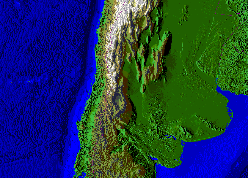
4. Chile – Historical Earthquake Activity: Using the chile10 view (with the chile10.hy4 catalog) in Seismic/Eruption, one can view the earthquake activity from January 1, 1900 to May 20, 2010 (Figures 1 and 2). The variation through time in data completeness (minimum magnitudes in the original catalogs – Centennial and USGS PDE) results in abrupt changes in the view at the beginning of 1964 and 1973. The February 27, 2010 M8.8 Chile earthquake and associated aftershocks also appears as two bursts of activity near the end of the time period. Also, note the great M9.5 Chile earthquake that occurred on May 22, 1960 (http://earthquake.usgs.gov/earthquakes/world/events/1960_05_22.php).
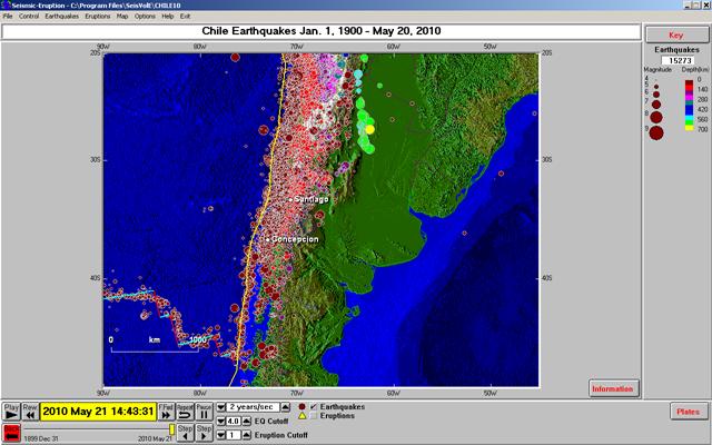
Figure 1. Seismic/Eruption view of chile10 area and earthquake
epicenters from the chile10.hy4 file.
The views (Figures 1 and 2) also
illustrate some classic plate tectonic boundaries. The west coast of South America is an
excellent example of a convergent boundary (shown by yellow lines on the
Seismic/Eruption displays) with associated mountain ranges (the Andes), deep
sea trench off the coast and earthquakes related to the subducting slab of
lithosphere (Figure 3; from This Dynamic
Earth – highly recommended introduction to plate tectonics). Notice the deep earthquakes (yellow and light
green epicenters) in the Seismic/Eruption views that are about 800 km to the
East of the West coast of South America.
A mid-ocean ridge and transform fault system (with associated shallow
earthquakes) is also visible in the southwestern corner of the chile10 view
(Figures 1 and 2). This mid-ocean ridge
system, which is the southern boundary of the Nazca plate which is moving
eastward and colliding with South America, continues west and connects to the
major Pacific Ocean mid-ocean ridge, the East Pacific Rise.

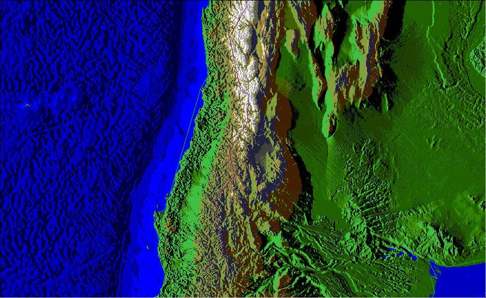
Figure 2. Enlarged Seismic/Eruption view of chile10
area (Figure 1) and earthquake epicenters from the chile10.hy4 file.
We
can view the earthquakes associated with that subduction zone along the west
coast of South America using the cross section tool in the Seismic/Eruption
software. Setting up the cross section
view is illustrated in Figure 4. The
white rectangle can be adjusted in size, azimuth (direction of the red profile
line), and position. In the subsequent
cross section view, all earthquake locations within the rectangle are projected
onto the vertical plane represented by the red profile and plotted (Figure
5). Instructions for making these cross
section diagrams with the Seismic/Eruption software and some example cross section
diagrams for various seismically active areas are available at http://web.ics.purdue.edu/~braile/edumod/sv/14cross.htm.
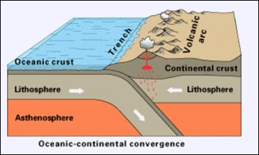
Figure 3. Schematic illustration of an oceanic plate –
continental plate convergent margin and subduction zone (from This Dynamic Earth: the Story of Plate Tectonics).
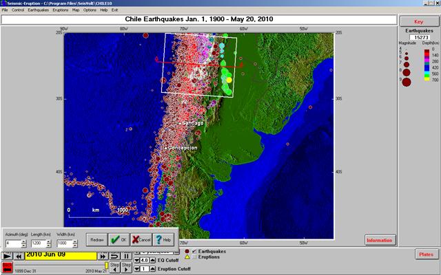
Figure 4. Seismic/Eruption view of chile10 area and earthquake
epicenters from the chile10.hy4 file and definition of the cross section view.
Notice that the subducted lithospheric slab beneath western South America dips at a fairly shallow angle to the East to a depth of about 200 km and then increases in dip angle and extends to about 650 km in depth. Also, we see that there are almost no hypocenters between about 300 and 500 km deep. What could be the cause of this gap in earthquake activity? It is possible that the slab slips into the mantle in aseismic deformation (continuous slow movement so that nor earthquakes occur), or perhaps the slab has broken and separated so that there is no subducted lithosphere (only normal mantle rocks) in this depth range. The answer to this question is not completely known. Maybe one of our students who examine this question using the Seismic/Eruption software will someday resolve this longstanding question.
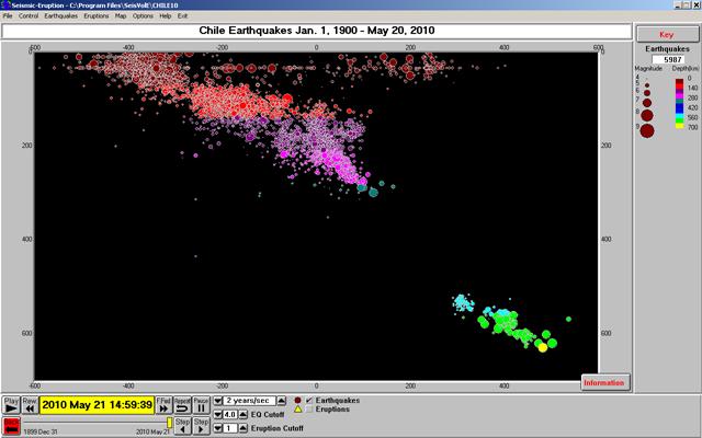
Figure 5. Cross section view of
earthquake hypocenters within the rectangular area shown in Figure 4. The horizontal scale is distance in
kilometers from the center of the rectangle along the profile (red line in
Figure 4). The vertical scale is depth
in kilometers. East is to the left. The apparent alignment of hypocenters at
about 35 km depth is an artifact caused by earthquake depths being assigned to
a default value when the depth cannot be accurately determined. A small number of other unusual locations
(“outliers”) are most likely caused by errors data or in the earthquake
location calculation.
Additional
seismicity maps and cross section diagrams that display earthquake locations (hypocenters)
associated with the subducted lithosheric slab beneath western South America
are shown in Figures 6 and 7. Advantages
of using the Seismic/Eruption program to display seismicity maps and cross
sections are that one can easily select the region of interest, the time period
and minimum magnitude to display, and the seismic activity can be seen through
time (in speeded up time). The software
also includes sound which allows the earthquake activity to be heard as
different pitched “beeps” (small magnitude events have a high pitched sound,
large earthquakes has a low pitched sound) and the time between events can also
be heard by how often the beeps occur.
You can control the audio through the Control pull down menu and the Earthquakes
pull down menu (Audio and Beeps Cutoff…).
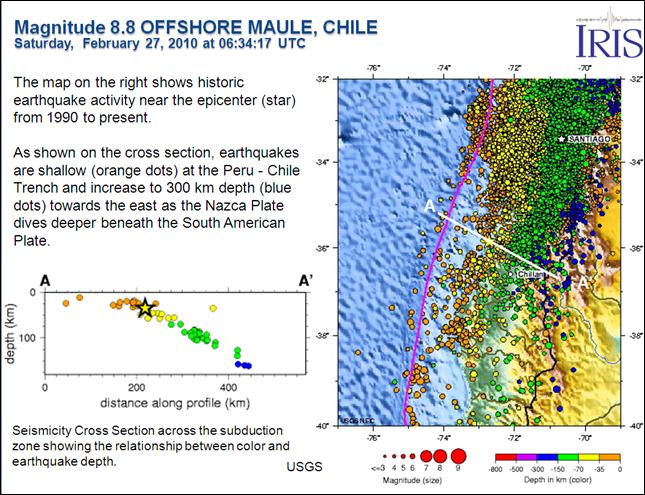
Figure 6. Seismicity in the coastal Chile area and
cross section view of earthquake hypocenters (powerpoint slide from Teachable
Moment materials of the IRIS Seismographs in Schools program, http://www.iris.edu/hq/retm, images from
the U.S. Geological Survey).
Figure 8 shows a
frequency-magnitude plot of earthquakes for the chile10 area. The frequency-magnitude plot using a linear
vertical scale is shown in Figure 8 and with a logarithmic vertical scale (the
standard way to plot the frequency-magnitude data) is shown in Figure 9. This is a classic and very useful earthquake
activity (seismicity) statistic. The
number of earthquakes greater than a given magnitude for the area and time
period selected are calculated and then divided by the number of years to
obtain the number of events equal to or greater than a given magnitude per
year. This number provides and average
number of events expected, for various magnitudes, per year. For example, in Figures 8 and 9, we see that
there have been about 25 M5+ earthquakes per year in the chile10 area so, based
on prior earthquake activity, we can expect an M5 or larger event about every
15 days. It is important to note that
this number is a statistical average and does not mean that there will be an
M5+ event at exactly every 15 days (periodic).
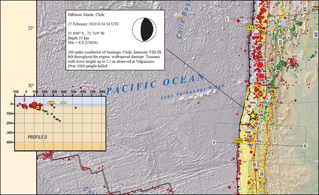
Figure 7. Seismicity in the coastal Chile area showing seismicity,
locations of source regions for significant historic events and cross section
view of earthquake hypocenters (extracted from USGS poster available at http://earthquake.usgs.gov/earthquakes/eqarchives/poster/regions/nazca.php).
Note
that by plotting the frequency-magnitude data on a linear vertical axis scale
(Figure 8) it is impossible to accurately represent the frequency of occurrence
of the larger magnitude earthquakes. It
appears that the numbers of events per year for magnitudes greater than about
6.5 are very close to zero. This is
true, but the actual numbers are impossible to estimate from the plot using the
vertical axis scale. Therefore, we
usually display frequency-magnitude data with a logarithmic vertical axis scale
as shown in Figure 9. The logarithmic
scale also displays the linear (straight line, with a negative slope)
relationship of the magnitudes and number of events of M+ per year. What would it mean if there was a positive
slope to this graph?
Uing
the data shown in Figure 9, “How many M6.5+ earthquakes per year would you
expect in this area?” [about one per year, “on the average”] “How many M8.6+ earthquakes?” [about 0.01 per
year, or one every 100 years, “on the average”].
We can use the Seismic/Eruption program to
easily calculate frequency-magnitude data such as shown in Figure 9. First, select an area (such as the chile10
area, although one can use any area including the entire world; the built-in
views in Seismic/Eruption and the chile10, chilega, chilecu and chileaf
views presented here are convenient areas; custom areas can be selected using
the Make Your Own Map option). Then, set
the time period of interest using the Set
Dates option from the Control pull down menu. Next, set the minimum magnitude on the EQ Cutoff
“dial” at the bottom of the screen. For
the chile10 area and catalog and 1973 or later, start at a cutoff of 4. Run Seismic/Eruption for this view (may need
to click on the Repeat button at the
bottom of the screen) and the counter in the upper right corner will display
the total number of events. Record the
results. Repeat the process for
magnitude cutoffs 4.5, 5.0, etc. The
frequency magnitude data can then be plotted on semi-log paper by hand (a
suitable template can be found in Figure 19.7 at http://web.ics.purdue.edu/~braile/edumod/sv/19excel.htm),
or using a data management and graphing program such as Excel (used to plot
Figures 8 and 9).
One
can plot the numbers of events for the entire time period or devide by the time
period to obtain the number of events per year as used in the plots in Figures
8 and 9.
In
calculating frequency-magnitude data, it is important to know the
characteristics of the earthquake catalog used.
For example, the mimimum magnitudes and completeness for various time
periods for the chile10 catalog were described above and are controlled by the
original data sources (USGS Centennial and PDE catalogs). For example, in Figures 8 and 9 we have
compared the frequency-magnitude data for large magnitude events for the
1973-2009 period (from the PDE catalog) with the data for the 1900-2009 period
(from the combined Centennial and PDE catalogs in chile10.hy4). Due to the longer time period of the
Centennial catalog, we would expect more accurate estimates of the number of
events for larger magnitudes. Notice
that the number of earthquakes per year, for magnitudes 7 and above for the two
time periods used, are quite similar.
In
calculating the frequency-magnitude data for the chile10 area, we have chosen
to include data through 2009 and not include the January 1 to May 20, 2010 data
as the earthquake record for this time period is dominated by the February 27,
2010 M8.8 earthquake and its aftershocks.
An
interesting frequency-magnitude exercise (not included here) would be to
calculate frequency-magnitude data for the 2010 earthquakes to see if the
classic frequency-magnitude relation (approximate straight line as shown in
Fiigure 9) exists for the aftershock data.
Because these results would be calculated for such a short time period
(less than five months), and the M8.8 earthquake and its aftershocks are
unusual events in the historic record, the number of earthquakes per year from
this calculation should not be used to estimate long term earthquake
probabilities. We will examine the M8.8
earthquake and aftershock sequence a later section.

Figure 8. Chile area frequency-magnitude plot using
linear vertical axis scale. Earthquake
data from Chile10 file (dots are for earthquakes January 1, 1973 to December
31, 2009 from the USGS PDE data; diamonds are for M7 and greater earthquakes
from January 1, 1900 to December 31, 2009 from the Centennial catalog and PDE
data; 20o to 48o S. latitude and 45o to
90o W. longitude).
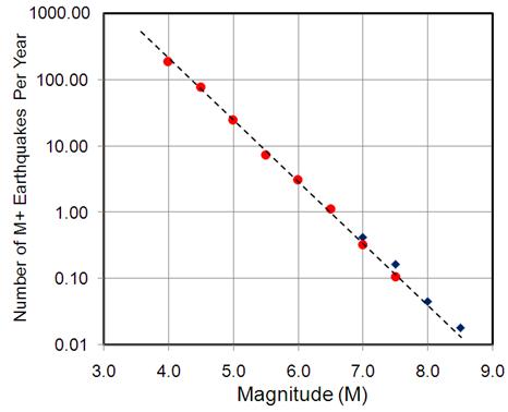
Figure 9. Chile area frequency-magnitude plot using
logarithmic vertical axis scale.
Earthquake data from Chile10 file (dots are for earthquakes January 1,
1973 to December 31, 2009 from the USGS PDE data; diamonds are for M7 and
greater earthquakes from January 1, 1900 to December 31, 2009 from the
Centennial catalog and PDE data; 20o to 48o South
latitude and 45o to 90o West longitude). The dashed line is an approximate best fit
straight line for the data.
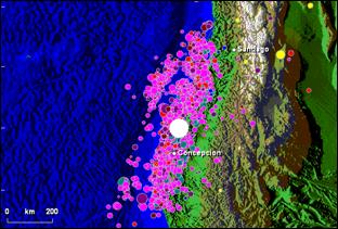
5. Chile – Seismic Gap: In this section, we will examine the larger earthquakes that have occurred in the central Chile area and the seismic gap that became apparent during the latter part of the 20th century. Earthquake epicenters from January 1, 1960 to February 26, 2010 with magnitudes of six or greater are shown in the Seismic/Eruption view in Figure 10. Notice that there are M6+ epicenters almost continuously along the coastline except for the “seismic gap” from just south of Santiago to Concepcion. The epicenters of the great 1960 M9.5 Chile earthquake and several large aftershocks can be seen just south of Concepcion. The continuity of M6+ earthquakes along almost all of coastal Chile (except for the seismic gap and the southernmost part of Chile) in the past 50 years (before the February 27 M8.8 earthquake) is also clearly visible using the chile10 view and selecting a time period of January 1, 1960 to February 26, 2010 and magnitude cutoff of six.
The Seismic/Eruption view in Figure 11 (January 1, 1960 to May 20, 2010, M6+) shows that the February 27, 2010 M8.8 earthquake and associated M6+ aftershocks occurred mostly within this gap. Seismic gaps have been described in many plate boundary areas around the world and are useful in identifying locations of likely future large earthquakes. Unfortunately, it is still difficult or impossible to accurately predict the time of major earthquakes that will occur in these gap regions. Research on the history of great earthquakes in the Chile area and the return period of these events is presented by Cisternas et al. (2005).
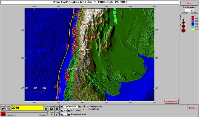
Figure 10. Chile area earthquakes of magnitude 6 and
greater for the period January 1, 1960 to February 26, 2010. Notice the gap in events from just south of
Santiago to Concepcion.
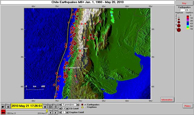
Figure 11. Chile area earthquakes of magnitude 6 and
greater for the period January 1, 1960 to May 20, 2010. The February 27, 2010 M8.8 earthquake and 23
M6+ aftershocks have virtually “filled”
the seismic gap.
Another
view of this sesimic gap is shown in Figure 12 based on the results of studies
by Beck et al. (1998). Note the source regions shown in Figure 12
for large coastal chile earthquakes and that the February 27 earthquake
occurred adjacent to source source zones that have not had major earthquakes in
recent years.
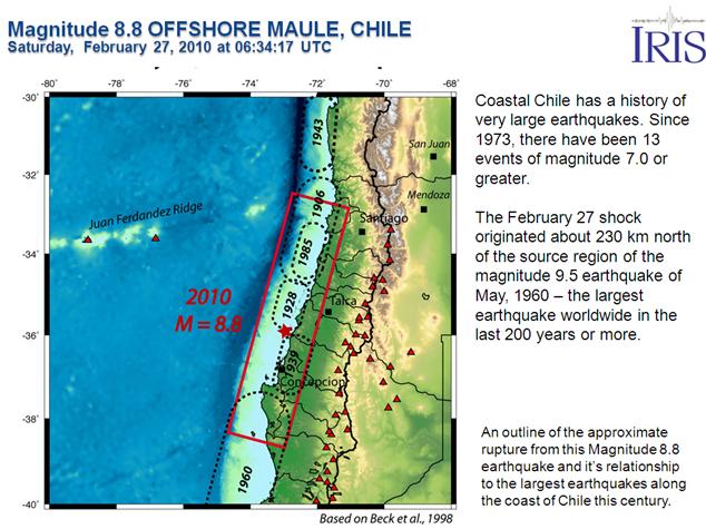
Figure 12. Seismic source regions for major earthquakes for the coastal chile area (powerpoint slide from Teachable Moment materials of the IRIS Seismographs in Schools program, http://www.iris.edu/hq/retm). Seismic source zones and gap (since 1939 event), for much of the source area of the 2010 earthquake, identified by Beck et al., 1998.
6. Closer view of Chile Earthquake Activity: Close-up views of the February 27, 2010 earthquake area and historical earthquake activity, including the seismic gap discussed in the previous section, are provided by the chilecu view. Using this view (January 1, 1960 to May 20, 2010, M6+) and setting the end date to February 26, 2010, the seismic gap in the area of the February 27th earthquake is very clearly seen (Figure 13). The same area, including the February 27 to May 20 events is shown in Figure 14.
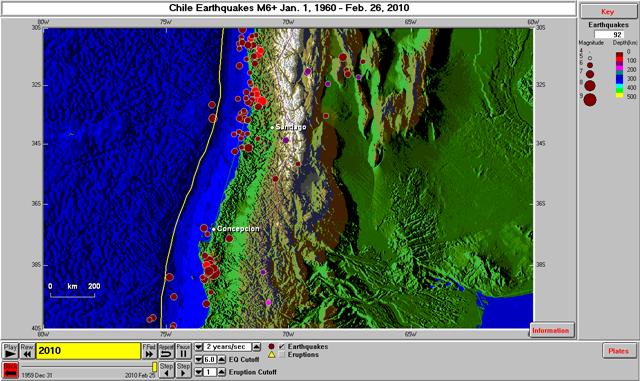
Figure 13. Chile area earthquakes of magnitude 6 and
greater for the period January 1, 1960 to February 26, 2010. Notice the gap in events from just south of
Santiago to Concepcion.
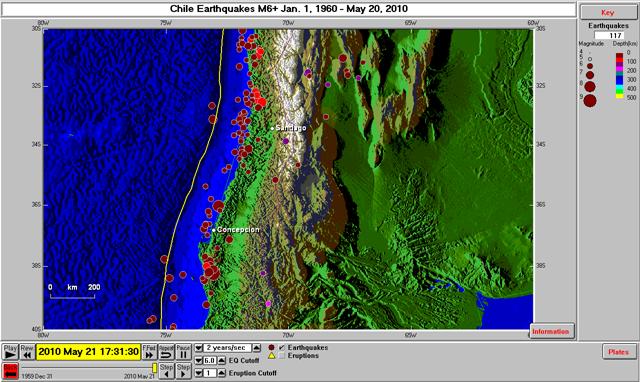
Figure 14. Chile area earthquakes of magnitude 6 and
greater for the period January 1, 1960 to May 20, 2010. The M8.8 February 27, 2010 earthquake and 23
M6+ aftershocks have virtually “filled” the seismic gap.
7. February 27, 2010 M8.8 Chile Earthquake Sequence: The Chile aftershock (chileaf) view is designed for exploring the earthquake activity in 2010, including the February 27th main shock earthquake and aftershocks. Figure 15 shows the 2010 earthquakes. There were thirteen earthquakes of magnitude 4 and greater in the selected area that occurred prior to the February 27, M8.8 event. Three earthquakes occurred on January 21, 2010 (maximum magnitude event was 5.1) close to the epicenter (within 70 km) of the February 27 main shock, but were not identified as foreshocks. Almost all of the epicenters in the view area that occurred after the February 27 main shock are aftershocks of the M8.8 earthquake or aftershocks of other large events (particularly the March 11, 2010 M6.9 aftershock) in the aftershock sequence. One can speed up or slow down the playback of earthquakes (use the speed dialog with up and down arrows near the bottom of the Seismic/Eruption view, and the Repeat button to restart the playback) to further examine the earthquake sequence.
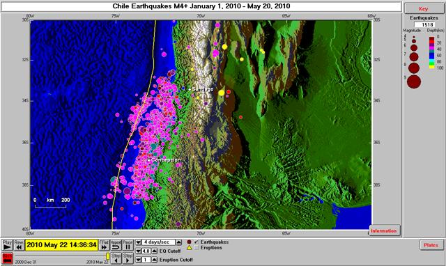
Figure 15. Chile area earthquakes of magnitude 4 and
greater for the period January 1, 2010 to May 20, 2010.
An
additional view of the 2010 earthquake sequence is shown in Figure 16. In this Figure, the epicenter of the February
27 main shock event is highlighted using a white dot (sizes of epicenter dots
are proportional to magnitudes of the events.
The legend for the dot size and magnitude is shown in the upper right
hand corner of the screen beneath the counter.
One can make changes in the magnitude scaling using the Magnitude Depth Scale… option in the Earthquakes pull down menu on the
Seismic/Eruption screen.
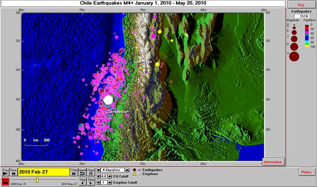
Figure 16. Chile area earthquakes of magnitude 4 and
greater for the period January 1, 2010 to May 20, 2010. The M8.8 February 27, 2010 main shock
earthquake is highlighted (using the Step
feature of the Seismic/Eruption program).
A
close-up view of the 2010 Chile earthquake sequence is shown in Figure 17. Notice
that the aftershocks define an approximately rectangular area. This area has been shown for many earthquakes
to be a good estimate of the fault area that ruptured during the main shock
event. Note that the main shock occurred
near the middle of this rupture zone so the rupture propagated to the north and
to the south – called bilateral rupture.
Some prominent past earthquakes have had initial rupture (and therefore
focus and hypocenter) at or near one end of the fault zone (unilateral
rupture). Earthquake ruptures of this
type include the great 1964 Alaska earthquake and the great 2004 Sumatra
earthquake. Details of the rupture type
and time history of the slip influence the radiated seismic energy and, for
very large shallow undersea or coastal earthquakes, the intensity and character
of tsunami generation.
Additional
details of the rupture area and slip history of the M8.8 February 27 earthquake
are provided in Figure 18 from finite fault modeling by Gavin Hayes of the U.S.
geological Survey.
If
we use the approximately rectangular area of the aftershocks (Figure 17) as an
indication of the fault plane that slipped during the February 27 main shock
event, we can make an estimate of the seismic moment and the moment magnitude
for this event. The moment is calcualted
from Mo = m x A x S, where
m is the shear modulus (strength) of
the rocks in the area of the fault and can be set at: ~40 GPa = 4.0 x 10¹¹
dynes/cm2
A is the
area of the fault plane (in cm2)
= ~180 x 700 km (from aftershock zone) = 1.26 x 1015 cm2
S is the average slip on the fault plane during
the earthquakes (estimated as 500 cm from the revised finite fault model from
Gavin Hayes shown in Figure 19).
Then,
Mo = (4 x 10¹¹ dynes/cm2
) x (1.26 x 1015 cm2) x (500 cm) = 2.52 x 1029
dyne-cm, which approximately corresponds to an M8.9 earthquake using the moment
magnitude equation Mw (or just M) = 2/3 log10(Mo) - 10.7
= 8.9. This value is close to the USGS official
magnitude of 8.8. Our estimate of moment
and therefore magnitude is dependent the estimate of average slip on the fault
from interpretation of Figure 19, and on the accuracy of our assumption and
measurement of the area of the fault plane from the aftershock area, and one
can see from Figure 17 that there is some uncertainty in interpreting that
area. Furthermore, the fault area
interpreted from seismological data by Hayes is somewhat smaller than the area
that we selected based on the aftershocks.
Nevertheless, the magnitude computed by this method is close to the
seismologically determined value.
For
more on moment magnitude, see http://earthquake.usgs.gov/learn/topics/measure.php,
and http://web.ics.purdue.edu/~braile/new/MomentMagnitude.ppt.
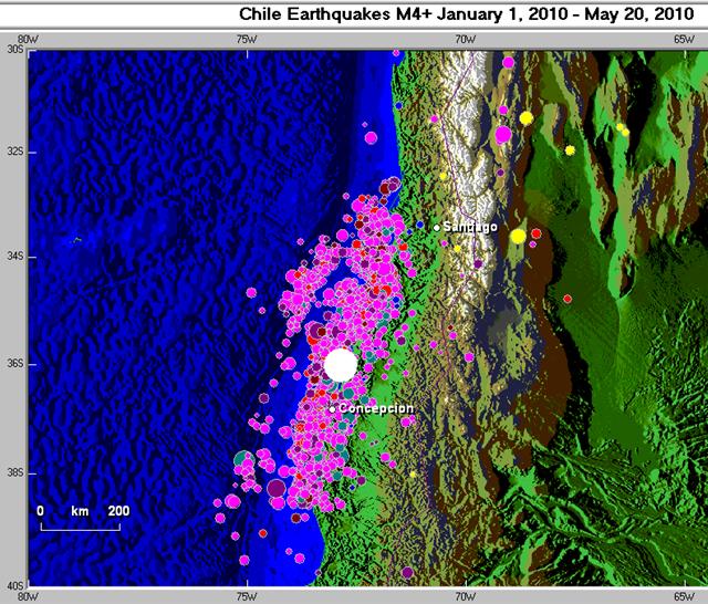
Figure 17. Close-up view of Chile area earthquakes of
magnitude 4 and greater for the period January 1, 2010 to May 20, 2010. The M8.8 February 27, 2010 main shock
earthquake is highlighted (using the Step
feature of the Seismic/Eruption program).

Figure 18. Seismic slip model for the M8.8 February 27,
2010 earthquake source region (powerpoint slide from Teachable Moment materials
of the IRIS Seismographs in Schools program, http://www.iris.edu/hq/retm; finite
fault modeling from Gavin Hayes, U.S. Geological Survey, http://earthquake.usgs.gov/earthquakes/eqinthenews/2010/us2010tfan/finite_fault.php).
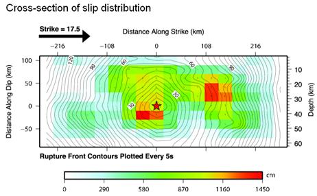
Figure 19. Finite fault modeling of the M8.8 February 27, 2010 Chile earthquake, interpreted slip distribution (from Gavin Hayes, U.S. Geological Survey, revised model, March 2010 http://earthquake.usgs.gov/earthquakes/eqinthenews/2010/us2010tfan/finite_fault.php).
We can further explore the 2010 Chile earthquake sequence by viewing the time history of the sequence in more detail using Excel graphs. In Figure 20, we have plotted all of the January 1 to May 20, 2010 M4+ earthquakes in the chileaf area as a function of time. The “normal” or background level of activity is visible for the period before February 27. The M8.8 main shock occurred on the 27th followed immediately by hundreds of aftershocks.
A close-up view of the main shock and aftershock sequence is shown in Figure 21. One can see that the aftershock activity has diminished somewhat with time both in number of events and the magnitude of aftershocks. However, the aftershock sequence will most likely go on for several months before the earthquake activity returns to pre-February 27 levels. And, as the graph shows, M6+ aftershocks have occurred unpredictably and throughout the sequence and have a high probability of occurring in the next few weeks or more.
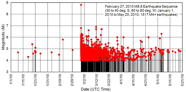
Figure 20. M8.8 2010 earthquake sequence, January 1, 2010 to May 20, 2010 – times of earthquakes shown by vertical lines; earthquake magnitude shown by dot. Only magnitude 4 and larger events shown.
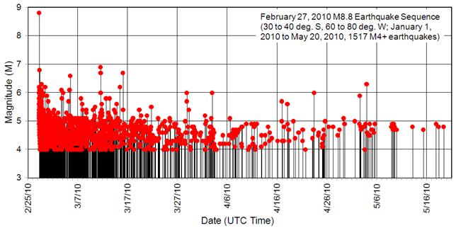
Figure 21. Close-up view of the M8.8 2010 earthquake sequence, January 1, 2010 to May 20, 2010 showing earthquakes after February 24, 2010 – times of earthquakes shown by vertical lines; earthquake magnitude shown by dot. Only magnitude 4 and larger events shown.
The 2010 Chile earthquake sequence is displayed in a slightly different way in the graph shown in Figure 22. In this Figure, the number of earthquakes per day (M4+) in the chileaf area is shown by the bold line and the maximum magnitude event for each day is shown by the red dot. There were 320 M4+ aftershocks on February 27 after the main shock event, followed by 224 aftershocks on February 28 and 103 aftershocks on March 1. The rapid decrease in number of aftershocks per day is very visible in the graph. However, although the maximum magnitude of aftershocks appears to be decreasing slowly, one cannot eliminate the possibility of M6+ aftershocks at least for the immediate future.
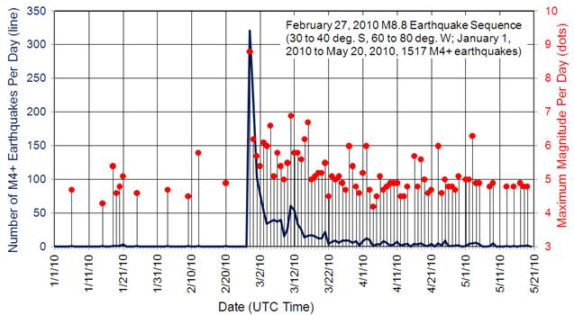
Figure 22. M8.8 2010 earthquake sequence, January 1, 2010 to May 20, 2010 – number of events per day shown by heavy line; maximum magnitude event for each day shown by dot attached to vertical line. Only magnitude 4 and larger events shown.
Shortly after the M8.8 February 27, 2010 Chile earthquake, members of the IRIS (Incorporated Research Institutions for Seismology, a seismology research and education consortium of academic institutions, http://www.iris.edu/hq/) community deployed 58 portable digital seismographs (Figure 23) in the Chile earthquake source zone area to provide detailed and high quality data for aftershocks. An example of some of the data recorded (seismograms) by the local network of seismographs is shown in Figure 24. Additional details on aftershock activity and the characteristics of aftershock earthquakes, including events of magnitude less than 4, will be available after research on the local network data has been completed.
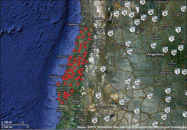
Figure 23. IRIS deployment of seismographs (~March 20 to
April 20, 2010) for monitoring aftershocks of the M8.8 February 27, 2010 Chile
earthquake.
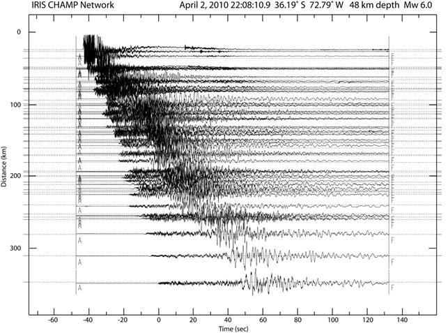
Figure 24. Seismogram record section for the M6.0 April
2, 2010 aftershock recorded by the IRIS network of seismographs (Figure 22) for
monitoring aftershocks of the M8.8 February 27, 2010 Chile earthquake. The seismograms are plotted versus relative
time and are arranged by epicenter to station distance. The epicenter of the April 2 earthquake was
about 18 km south of the location of the February 27 main shock event.
8. Chile Earthquake Hazards and Damage: The M8.8 February 27, 2010 Chile earthquake caused considerable loss of life, damage to structures from severe shaking of the ground, and damage to coastal cities and towns from the tsunami that was generated by vertical movement of the sea bottom caused by the earthquake fault slip and release of stored elastic energy. Some examples of earthquake damage in Chile are shown in the photographs in Figure 25.
|
|
|
|
|
|
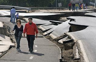
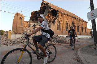
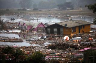
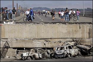
Figure 25. M8.8 February 27, 2010 Chile earthquake damage photos.
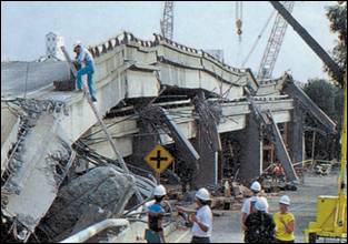
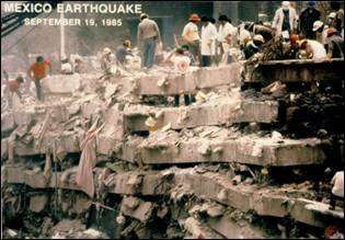
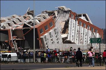
Occasionally, earthquakes can cause catastrophic damage, particularly from complete or near complete collapse of structures or from very large tsunami such the December 26, 2004 Sumatra tsunami. Some examples of catastrophic or near catastrophic earthquake damage from previous large quakes are shown in Figure 26.
An additional and unusual example of catastrophic earthquake damage was caused by the M8.8 February 27, 2010 Chile earthquake – a building that toppled like a felled tree. The Alto Rio apartment building in Concepcion, Chile failed at its base and fell over essentially in one piece and then broke into two large pieces when it hit the ground (Figure 27). Eight people were killed in the building, but amazingly, 79 people in the building survived the fall to the ground, including a father and daughter in their apartment on the thirteenth floor (their story was widely reported in the news, http://seattletimes.nwsource.com/html/nationworld/2011216614_apltchilesurvivorsstory.html).
An additional view of the Alto Rio building, in two parts, on the ground is shown in Figure 28. The failed bottom floor of the structure (above two underground parking garages) is shown in the photograph in Figure 29.
A fun educational activity for learning about how
structures respond to earthquake shaking is the building contest (http://web.ics.purdue.edu/~braile/edumod/building/building.htm). In this activity, students construct model
buildings that are tested for their resistance to damage from shaking using a
simple shake table. Various modes of
building failure are usually evident in some of the model buildings. One can then improve the building design and
re-test the structures.
|
|
|
|
|
|
|
|
|

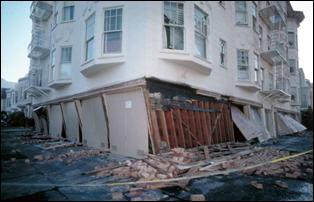
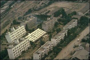
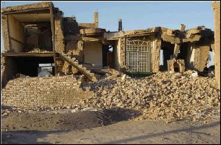
Figure 26. Examples of catastrophic or near catasrophic earthquake damage. Upper left: Collapse of elevated roadway, Oakland, California, M6.9 Loma Prieta earthquake, October 18, 1989. Upper right: Catasrophic collapse (“pancaking”) of multistory building in Mexico City caused by an M8.0 earthquake from near the coast of Michoacan, Mexico, September 19, 1985. Middle left: Apartment buildings in Niigata, Japan that tilted and sunk into the ground due to liquefaction caused by an M7.5 earthquake on June 16, 1964. Middle right: Almost complete collapse of three story unreinforced masonry building; M6.6 Bam, Iran earthquake of December 26, 2003. Lower left: Damage from the December 26, 2004 Sumatra tsunami caused by an M9.0 earthquake. Lower right: Nearly collapsed four story apartment building damaged by the M6.9 Loma Prieta earthquake, October 18, 1989. The damage is an example of “soft first story” failure.
|
|
|

Figure 27. Catastrophic earthquake damage to the Alto
Rio building, Conception, Chile due to the February 27, 2010 M8.8
Earthquake. Left: Rio Alto apartment
building before earthquake (from: http://nbo.icann.org/meetings/nairobi2010/presentation-chilean-earthquake-08mar10-en.pdf). The earthquake caused the building to topple
toward the back of the building, toward the left in the photo. Right: Toppled Alto Rio building; the top
level of the building is in the left foreground.
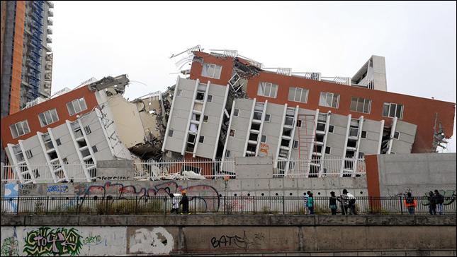
Figure 28. Catastrophic earthquake damage to the Alto Rio building, Conception, Chile due to the February 27, 2010 M8.8 Earthquake. The base of the toppled building is to the right.
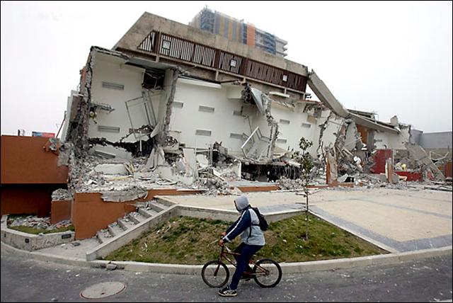
Figure 29. Catastrophic earthquake damage to the Alto Rio building, Conception, Chile due to the February 27, 2010 M8.8 Earthquake. Photo shows the base of the toppled building.
9. References:
Beck, S. L., S. Barrientos, E. Kausel, and M. Reyes (1998). Source characteristics of large historic earthquakes along the Chile subduction zone, J. S. Am. Earth Sci. 11 (2) 115-129. (download 1.3 MB, http://www.geo.arizona.edu/web/Beck/pubs/Beck_etal_1998.pdf)
Cisternas, M., and fourteen other authors, Predecessors of the giant
1960 Chile earthquake, Nature 437,
404-407 (15 September 2005), abstract available online at:
http://www.nature.com/nature/journal/v437/n7057/abs/nature03943.html
U.S. Geological Survey, This Dynamic Earth: the Story of Plate Tectonics, online edition, http://pubs.usgs.gov/gip/dynamic/.