Voyage Through Time – A

Plate Tectonics Flipbookã

Larry Braile, Professor

Purdue University

http://web.ics.purdue.edu/~braile

Sheryl Braile, Teacher

Happy Hollow School

April, 2000

Objectives: To view the breakup of the super-continent Pangea over the past 190 million years and chart the subsequent movement of landmasses, and to better understand plate tectonics. (This lesson plan was adapted from a similar activity by Ford, 1994. A similar flipbook is presented in Tremor Troop (2000). Additional information on plate tectonics and continental drift can be found in Bolt, 1993; Ernst, 1990; and the USGS publication "This Dynamic Earth: The Story of Plate Tectonics" [also available on the Internet at: http://pubs.usgs.gov/publications/text/dynamic.html].)

Materials:

Each student will need:

- a copy of the map sheets (on card stock for Figures 1A to 1E)

- colored pencils or crayons: red, orange, yellow, green, blue, purple, tan

- scissors

- access to a world map showing terrain, such as mountains and seafloor (an excellent map for this purpose is This Dynamic Planet, Simkin et al., 1994, 1:30,000,000 scale. To order, call the U.S. Geological Survey Map Distribution at 1-888-ASK-USGS; http://pubs.usgs.gov/pdf/planet.html.)

Procedure:

1. Provide students with copies of map sheets (Figure 1) photocopied on heavy paper (card stock), each with a number of frames (F1 to F20). These frames are reconstructed maps of the landmasses that existed on Earth at a specific time. The interval between successive frames is 10 million years (mya = millions of years ago). Frame 20 depicts landmasses as they are today. The maps are a view (projection) of the entire Earth, showing the outline of the continents, onto a flat surface. The orientation and representation of the Earth’s continental regions can be most easily visualized by looking at map F20 (present day view) in Figure 1E. On this and the other maps, the equator (zero degrees latitude) would be a horizontal line through the middle of the map area (through northern South America, central Africa and Indonesia). Similarly, the Prime Meridian (zero degrees longitude) would be a vertical line through the middle of the map area (through England, Spain and western Africa).

2. Beginning with frame 20 and working back-wards, have students identify the landmasses listed in the table below. Have student groups color these landmasses as indicated in the table, assigning a different land mass to each student group. Have students continue working backwards through the frames until they can no longer identify the individual landmasses. By assigning different land masses to different groups, the students will be able to share their results when the flip books are completed and several different continental movements and plate tectonic interactions will be illustrated on the different flip books.

Land Masses Color

North and South America Yellow

Australia Tan

India Orange

Africa Green

Europe and Asia Red

Antarctica Blue

Greenland Purple

3. An option for coloring the landmasses is to select more than one continent that will display a particular movement and interaction through time. For example:

a. Begin with F1 (190 mya) and color the super-continent Pangea green. Continue to identify and color Pangea on subsequent frames until the continents are completely separated (F15)

b. Working backwards through time (begin with F20), select two continents that display a particular plate tectonics interaction and color the continents on the frames back through time until the continents are together. Good examples are Africa and South America or Europe and North America that illustrate continental separation (divergent plate boundaries) and opening of the Atlantic Ocean basin through time, or India and Asia that shows a continental collision (convergent plate boundary).

4. Have students cut out each frame carefully along the outside frame lines. When all rectangles are cut out, stack them in order 1-20. Frame 1 should be on top (although the frames could also be ordered so that F20 is on the top, but it is useful to have all the flip books have the same order to minimize confusion as students share their individual flip books). Booklets should then be carefully aligned and stapled securely along the left side. A heavy-duty stapler will work best with the card stock. Alternatively, small binder clips can be used.

5. Holding the rectangles along their left side, have students flip through the frames, observing changing position of the landmasses (plate movement and continental drift). They are modeling the breakup of Pangea and the movement of landmasses over 190 million years, arriving at the configuration of our present-day continents.

6. Encourage student groups to exchange and view various flipbooks in order to make observations and inferences from the movements of the different continents.

Have students consider the following questions:

1. What event began to occur about 190 million years ago?

2. During your coloring of the frames, in which frame did you locate the first appearance of the following landmasses:

North America?

Australia?

India?

Europe?

Antarctica?

3. In which frame did you locate the final breakup of Pangea? Why did you choose that frame and not another?

4. Sometimes when two plates collide, the landmasses (continents) within the plates are pushed together and a mountain range can form. Using a world map, identify two locations where mountain ranges exist and where you hypothesize plate collisions between continents or parts of continents have occurred. Use your flipbooks to confirm your hypothesis. (Note that not all present-day mountain ranges were formed by continental collision events or by plate convergence that occurred during the last 190 million years.)

5. If mountain ranges can form where plates are colliding, what would you hypothesize might occur where plates are separating? Apply your hypothesis to identify locations on a world map where plates might be separating (both oceanic and continental lithospheric plate divergence zones can be identified on the map and in the flip books). The flipbooks will help you identify previous plate separations.

Extension Activities:

1. Using selected frame sheets (Figure 2), have students color the land mass identified as India today on each of the frames. Have students graph the changing position of India’s landmass (distance from the equator by identifying the latitude of the approximate center of India through time; the latitude scale on Figure 2A should be used to estimate the latitude of India on each frame) over time, using the provided graph paper (Figure 3). The equator is the horizontal line on the maps in Figure 2. Note the probable effects on climate of India through the past about 100 million years (paleoclimate) as India’s position has changed. How would this climate be different then the climate in India today? Can you find any evidence (in available books or reference materials or in an Internet search) that supports the concept of a different climate for India 100 or more million years ago? Students could choose a different land mass and repeat this graphing activity to compare movement over time.

2. Repeat the previous activity having students measure and plot the opening of the Atlantic ocean through time. Select two locations on opposite sides of the Atlantic on Frame 20 on Figure 2B (present or 0 mya map). Suggested points in the north Atlantic are: the northeastern US on the east coast of North America and the Iberian peninsula (Spain) on the west coast of Europe. Suggested points for the south Atlantic are the easternmost point along the east coast of South America (eastern Brazil) and the prominent indentation along the west coast of Africa near Nigeria. Referring to these points on a world map or on a transparency of Figure 2B on an overhead projector may be useful.

Measure the distance between these points using the kilometer scale provided on Figure 2A. Plot the distance between the two points, showing the opening of the Atlantic through time, on the graph provided in Figure 4. It will be easiest to work backwards (beginning with Frame 20) through time. You should be able to recognize a separation between your two points back to about 80 to 120 million years ago. As a challenge, calculate the approximate average speed (say in km/million years) for the opening of the Atlantic inferred from your graph. How does this speed compare with typical plate velocities (1-15 cm/yr) that are inferred for contemporary plate tectonic motions (you will need to make a conversion between km/million years and cm/yr in order to make the comparison)?

3. View plate tectonic reconstructions through time (continental drift) on commercial videotapes ("Miracle Planet -- The Heat Within" shows collision of India and Asia; "Continental Drift and Plate Tectonics" by Prof. Tanya Atwater [recommended]; or "Planet Earth -- The Living Machine"; or "National Geographic -- Born of Fire"), CD-ROM or Videodisk ("The Great Ocean Rescue" -- Tom Snyder productions -- 1-800-342-0236), a computer program ("Time Machine Earth", 1991, Sageware Corporation, 1282 Garner Ave., Schenectady, NY, 12309, 1-518-377-1052), or using commercial flip books (see reference below). For additional information on finding resources related to this activity and the videotapes, see Seismology-Resources for Teachers (http://web.ics.purdue.edu/~braile/edumod/seisres/seisresweb.htm). Several plate tectonic animations are also available on the Internet; some addresses are:

http://www.ucmp.berkeley.edu/geology/tectonics.html.

http://www.scotese.com/earth.htm

http://wrgis.wr.usgs.gov/docs/usgsnps/animate/pltecan.html

http://www.geol.ucsb.edu/~atwater/Animations/Animations-FR.html

http://www.odsn.de/odsn/services/paleomap/animation.html

http://www.ig.utexas.edu/research/projects/plates/plates.htm#movies

http://www.uky.edu/ArtsSciences/Geology/webdogs/plates/reconstructions.html

http://www.seismo.unr.edu/ftp/pub/louie/class/333/atwater/

References:

Atwater, Tanya, Continental Drift and Plate Tectonics, 20 minutes videotape, 1988.

(send $15 check payable to the Regents of the University of California, to:Rick Johnson, Instructional Consultation, University of California, Santa Barbara,

Santa Barbara, CA 93106).

Bolt, B.A., Earthquakes and Geological Discovery, W.H. Freeman, New York, 229 pp., 1993.

Continental Drift Flipbooks, (10-pack $40 + $3 S&H, payment must accompany order)

Geosociety, University of Texas at Arlington, PO Box 19049, Arlington, TX 76019,

FAX: 817-273-2628.

Ernst, W.G., This Dynamic Planet, Columbia University Press, New York, 281 pp., 1990.

Ford, B.A., Project Earth Science: Geology, National Science Teachers Association,

Washington, D.C., 1994.

Simkin, T., J. D. Unger, R. I. Tilling, P. R. Vogt, and H. Spall, This Dynamic Planet – World

Map of Volcanoes, Earthquakes, Impact Craters, and Plate Tectonics, Smithsonian

Institution and U.S. Geological Survey, 1994. ($7 + $5 shipping and handling, payment must accompany order, U.S. Geological Survey, Map Distribution, Federal Center, PO Box 25286, Denver, CO 80225, 1-888 ASK-USGS,

http://pubs.usgs.gov/pdf/planet.html.

Tremor Troop – Earthquakes: A Teacher’s Package for K-6, NSTA/FEMA, FEMA 159, Revised

Edition, August, 2000. (available from FEMA Publication Warehouse, 1-800-480-2520).

U.S. Geological Survey, This Dynamic Earth: The Story of Plate Tectonics, ($6 payment must accompany order), U.S. Geological Survey, Map Distribution, Federal Center, PO Box 25286, Denver, CO 80225, 1-888 ASK-USGS, http://pubs.usgs.gov/publications/text/dynamic.html

				Figure 1. Frames F1 through F20 showing the configuration of the continents on a projection of the Earth (the equator would be a horizontal line through the middle of the map; the prime meridian would be a vertical line through the center of the map) from 190 million years ago (mya) through the present. A. Frames F1 to F4. B. Frames F5 to F8. C. Frames F9 to F12. D. Frames F13 to F16. E. Frames F17 to F20. Figure 1A.
				Figure 1. Frames F1 through F20 showing the configuration of the continents on a projection of the Earth (the equator would be a horizontal line through the middle of the map; the prime meridian would be a vertical line through the center of the map) from 190 million years ago (mya) through the present. A. Frames F1 to F4. B. Frames F5 to F8. C. Frames F9 to F12. D. Frames F13 to F16. E. Frames F17 to F20. Figure 1A.
		Figure 1. Frames F1 through F20 showing the configuration of the continents on a projection of the Earth (the equator would be a horizontal line through the middle of the map; the prime meridian would be a vertical line through the center of the map) from 190 million years ago (mya) through the present. A. Frames F1 to F4. B. Frames F5 to F8. C. Frames F9 to F12. D. Frames F13 to F16. E. Frames F17 to F20. Figure 1B.
Figure 1. Frames F1 through F20 showing the configuration of the continents on a projection of the Earth (the equator would be a horizontal line through the middle of the map; the prime meridian would be a vertical line through the center of the map) from 190 million years ago (mya) through the present. A. Frames F1 to F4. B. Frames F5 to F8. C. Frames F9 to F12. D. Frames F13 to F16. E. Frames F17 to F20. Figure 1C.
			Figure 1. Frames F1 through F20 showing the configuration of the continents on a projection of the Earth (the equator would be a horizontal line through the middle of the map; the prime meridian would be a vertical line through the center of the map) from 190 million years ago (mya) through the present. A. Frames F1 to F4. B. Frames F5 to F8. C. Frames F9 to F12. D. Frames F13 to F16. E. Frames F17 to F20. Figure 1D.
	Figure 1. Frames F1 through F20 showing the configuration of the continents on a projection of the Earth (the equator would be a horizontal line through the middle of the map; the prime meridian would be a vertical line through the center of the map) from 190 million years ago (mya) through the present. A. Frames F1 to F4. B. Frames F5 to F8. C. Frames F9 to F12. D. Frames F13 to F16. E. Frames F17 to F20. Figure 1E.
				Figure 2. Selected maps for measuring the positions of continental regions through time. The horizontal line through the center of the map is the equator. A. Frames F8, F10 and F12. Scales at the bottom of the figure are for determining latitude and measuring distances between two landmasses. B. Frames F14, F16, F18 and F20. Figure 2A.
				Figure 2. Selected maps for measuring the positions of continental regions through time. The horizontal line through the center of the map is the equator. A. Frames F8, F10 and F12. Scales at the bottom of the figure are for determining latitude and measuring distances between two landmasses. B. Frames F14, F16, F18 and F20. Figure 2B.

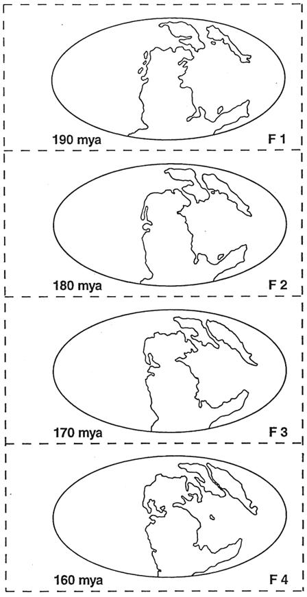
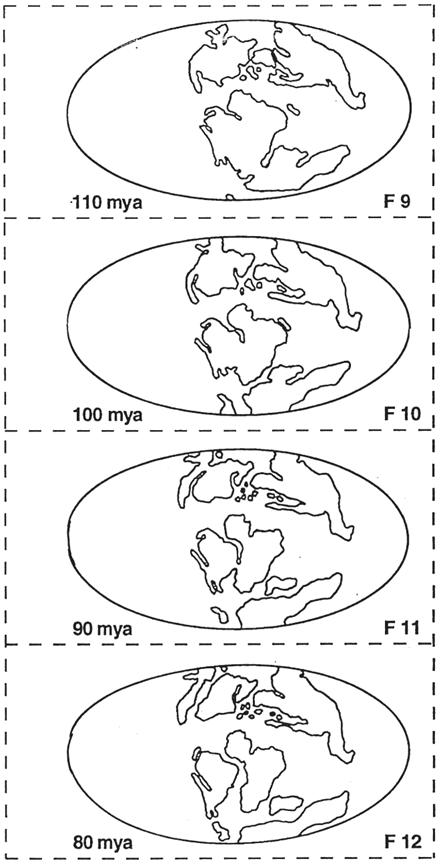
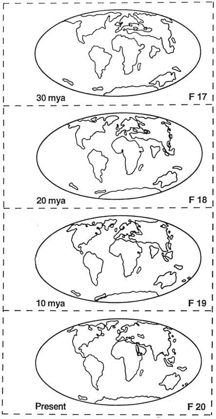
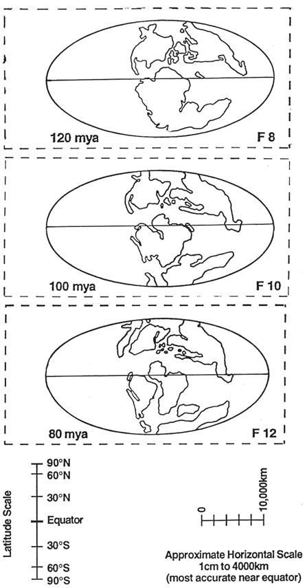
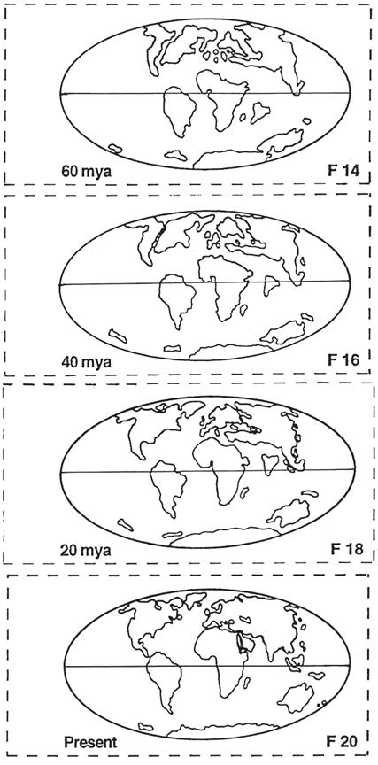
Figure 3. Graph for plotting position (latitude) of a continent (India, for example) through time.

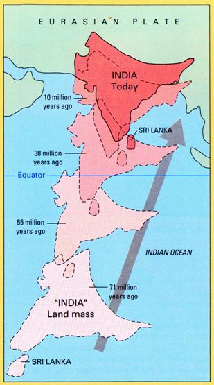
Figure 4. The movement of the Indian subcontinent through time by plate tectonics motions (from USGS, "This Dynamic Earth – The Story of Plate Tectonics").

Figure 5. Graph for plotting distance between two continents through time as the Atlantic Ocean basin opened.