Background:
Examine
the seismograms shown in Figure 1. The
display is called a seismic record section.
Each trace is a seismogram recorded at a seismograph station. Most of the station locations (letter code
adjacent to each trace) can be found on the seismograph network maps shown in
Figures 2 and 3. On the record section
(Figure 1), the seismograms are plotted according to the distance (in degrees,
geocentric angle) from the earthquake location and time from the earthquake
origin. The traces are of the vertical
component of ground motion, and have been filtered to include only periods
longer than 125 seconds. The prominent
arrivals (often called phases) that “angle across” the record section and are
labeled R1, R2 and R3 are long-period Rayleigh (surface) waves that travel
along the surface of the Earth. Surface
waves penetrate (have particle motion) to depths of tens to hundreds of km
(depending on the type of wave and the period of oscillation of the phase) but
travel approximately parallel to the Earth’s surface.
Questions:
1. What explains the unusual
pattern of the R1, R2 and R3 phases across the record section? (That is, what are the surface wave
propagation paths for R1, R2 and R3 that explain this pattern?). Hint:
For our purposes we can assume that all of the stations are located in a
line (actually a great circle) around the Earth. The cross section diagram in Figure 4
illustrates this situation. A few of the
seismograph stations are shown at the appropriate distance from the
earthquake. (The actual locations of the
stations are shown in Figures 2 and 3 and are not arranged in a line or great
circle path through the epicenter of the Loma Prieta Earthquake. However, because the surface waves propagate
in all directions from the source, the arrival times are approximately the same
as if the stations were all located along a great circle path from the
epicenter.)
2. What is the approximate
velocity of propagation of the long period Rayleigh waves illustrated in Figure
1? Hint:
the velocity along the surface (often called the apparent velocity,
which for the surface waves is the actual propagation velocity because they are
propagating parallel to the surface) can be determined from the slope (velocity
= 1/slope) of the arrivals for the R1, R2 and R3 phases on the record
section. What is the velocity in
degrees/minute? For the spherical Earth
of approximate radius 6371 km, one degree of geocentric angle corresponds to a
distance along the surface of approximately 111.19 km. Using this information, what is the
approximate velocity of the long-period Rayleigh waves in units of
kilometers/second? (The conversion to
km/s is useful because these units are commonly used to describe the velocity
of propagation of seismic waves through Earth materials.)
3. Using the velocity found in
question 2 (in degrees/minute or km/s), how long does it take for the long
period Rayleigh wave to propagate completely around the Earth (360 degrees)?
Reference
(and source of Figures 1, 2 and 3, pp. 14, 189, 190):
Lay, Thorne, and Terry C. Wallace, Modern
Global Seismology, Academic Press, San
Diego, California,
521 pp., 1995.
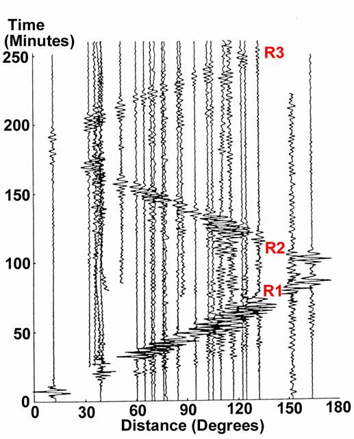
Figure 1.
Seismograms of the 1989 Loma Prieta (central California) earthquake in record section
form showing the long period Rayleigh wave (largest amplitudes) labeled R1, R2,
R3. The seismograms are vertical
component records and have been filtered to include only periods longer than 125
seconds. Seismograph stations that
recorded the seismograms, in order of distance, are: AMNO, COL, KIP, HRV, SJG, PPT, RPN, AFI, CAY,
MDJ, HIA, TOL, BDF, WMQ, TAM, KMY, CAN, TWO, HYB, BCAO, NWAO, SLR, RER. Locations of most of these stations are shown
on the maps in Figures 2 and 3.
(Modified from Lay and Wallace, 1995).
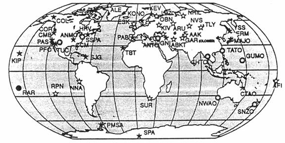
Figure 2.
Locations of modern, digital, broadband seismograph stations of the
IRIS/USGS-GSN and IRIS-IDA networks.
(Modified from Lay and Wallace, 1995).

Figure 3.
Locations of modern, digital, broadband seismograph stations of the
Project GEOSCOPE network. Dots and
triangles are GEOSCOPE stations. Open
circles are other digital stations recording seismograms shown on the record
section in Figure 1. (Modified from Lay
and Wallace, 1995).

Figure 4.
Schematic diagram illustrating a cross section through the Earth and the
locations of seismograph stations.
Distance from the earthquake epicenter to a station can be measured in
kilometers along the surface or by the geocentric angle (D) in
degrees.