EAS 557
Introduction to Seismology
Robert L. Nowack
Lecture 10
Equation of Motion in an Unbounded Medium: Plane Waves
The equation of motion for a linear, isotropic, and elastic solid can be written as
![]()
or in vector form,
![]()
where ![]() and
and ![]() are the Lamé constants,
are the Lamé constants, ![]() is the particle
displacement, and
is the particle
displacement, and ![]() is the force term.
is the force term.
We can use the formulation of Helmholtz
to decompose ![]() (and
(and
![]() ) into scalar and vector potentials. Let
) into scalar and vector potentials. Let ![]() , where
, where ![]() and
and ![]() , where
, where ![]() , then
, then
which are simple wave equations. We will first look at the simple wave equation without the source term. Consider,
In order to solve this equation, we will use the technique of separation of variables.
Assume a solution in the form
![]()
then,
This results in,
where ![]() is an arbitrary
constant. We have chosen the sign in
anticipation of the form we want. Since
the left term is only a function of
is an arbitrary
constant. We have chosen the sign in
anticipation of the form we want. Since
the left term is only a function of ![]() and the right term is
only a function of t, they both must
be equal to a constant and can be solved separately.
and the right term is
only a function of t, they both must
be equal to a constant and can be solved separately.
1) ![]() . A solution of this is
. A solution of this is ![]() , with
, with ![]() and
and ![]() where
where ![]() is radial frequency in
rad/sec.
is radial frequency in
rad/sec.
2a) For the 1-D case,  . A solution of this
is of the form
. A solution of this
is of the form ![]() where
where ![]() is
the spatial wavenumber in radians per km.
is
the spatial wavenumber in radians per km.
The combined
solution is of the form ![]() . General solutions can
be written as
. General solutions can
be written as  . Our sign convention
uses a combined form
. Our sign convention
uses a combined form ![]() with a plus sign for
the kx term
and a minus sign for the
with a plus sign for
the kx term
and a minus sign for the ![]() term.
term.
2b) For the 3-D case,
![]()
![]()
![]()
then,
 and
and ![]()
where
The wavenumber vector can then be written ![]() where
where
![]()
Thus, we have a combined solution of the
form ![]() which is called a
plane wave solution. General solutions
can be written as
which is called a
plane wave solution. General solutions
can be written as
where ![]() is the weighting
function for the
is the weighting
function for the ![]() term and k3 is defined above.
term and k3 is defined above. ![]() must
be chosen to satisfy the boundary conditions and initial conditions.
must
be chosen to satisfy the boundary conditions and initial conditions.
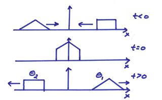
We will look at the solution to the wave equation in a slightly different way for the 1-D case. Let
We will postulate a solution of the
form ![]() (D’Alembert’s
solution in 1-D) where
(D’Alembert’s
solution in 1-D) where ![]() and
and ![]() are arbitrary
functions of the combined variable
are arbitrary
functions of the combined variable ![]() .
. ![]() is
a function that has a fixed shaped and for increasing t moves in the +x
direction and
is
a function that has a fixed shaped and for increasing t moves in the +x
direction and ![]() is a function that has
a fixed shape and moves in the –x
direction for increasing t.
is a function that has
a fixed shape and moves in the –x
direction for increasing t.
We verify that this is the solution by letting ![]() where
where
![]() . Then by the chain
rule
. Then by the chain
rule
![]()
and

Also,
![]()
and
Then, we see that ![]() is a solution of the
simple wave equation for any functional shape that moves in an undistorted
fashion to the right at a special
is a solution of the
simple wave equation for any functional shape that moves in an undistorted
fashion to the right at a special ![]() . Thus,
. Thus,
Doing the same for ![]() and adding, then
and adding, then
![]()
Thus, the above form satisfies the wave equation.
Thus, the simple
wave equation in 1-D has two solutions which propagate undeformed
in opposite directions with increasing t
with a velocity ![]() . This is one of the
fundamental properties of waves. The
solution can be written as disturbances that propagate at well-defined
velocities.
. This is one of the
fundamental properties of waves. The
solution can be written as disturbances that propagate at well-defined
velocities.
Let the right propagating solution be
![]()
which is the right propagating cosine wave, or in complex notation
![]()
which is the same as the previous
solution derived using separation of variables and is sinusoidal over all x and t, where ![]() .
.
Let
k = wavenumber = ![]() in rad/km
in rad/km
with ![]() = wavelength. Also,
= wavelength. Also,
![]() = angular frequency =
= angular frequency = ![]() in radian/sec
in radian/sec
with T = period. The wavelength ![]() and the period T are
shown below.
and the period T are
shown below.
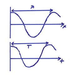
At a fixed time, say t = 0,
as a function of x then
At a fixed x, say x = 0,
as a function of t then
The wave equation also requires that k and ![]() be related through the
wave speed
be related through the
wave speed ![]() as
as
![]()
Alternatively, this can be written as
![]()
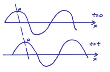
From the figure above, we can
choose any point A of constant phase ![]() and this propagates
with velocity
and this propagates
with velocity ![]() . The following
properties can be inferred:
. The following
properties can be inferred:
1) A sinusoidal wave solution is completely nonlocalized in space (as well as time). In this sense it is in steady state. Its propagating nature can be isolated by following a given peak or trough.
2) Arbitrary solutions can be written as a superposition of sines and cosines or (complex exponentials). Thus,
which can be thought of as a Fourier synthesis of sinusoidal wave solutions to construct more general solutions.
A plane wave solution in three dimensions can be written
![]()
where A is the amplitude and ![]() is the phase. The wavenumber vector is
is the phase. The wavenumber vector is ![]() and
and ![]() . Also,
. Also, ![]() ,
, ![]() ,
, ![]() where
where
![]()
For example, for some fixed time in 2-D then
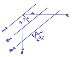
where in the figure ![]() ,
, ![]() ,
, ![]() and
and ![]() . Then
. Then ![]() are the apparent
wavelengths in the x = x1, and z = x3
directions, i
equals the angle from vertical,
are the apparent
wavelengths in the x = x1, and z = x3
directions, i
equals the angle from vertical, ![]() ,
, ![]() , and
, and ![]() , and
, and ![]() . Also,
. Also,
![]()
The wavenumber vector can be written
Let ![]() be a unit vector in
the plane of constant phase (wavefronts)
be a unit vector in
the plane of constant phase (wavefronts) ![]() , then
, then
![]() , Thus, the wave
vector
, Thus, the wave
vector ![]() is perpendicular to the
wavefront.
is perpendicular to the
wavefront.
Since velocities are related to wavelengths by  (since
 ![]() is related to
particular peaks and troughs, it is called the “phase velocity”), the apparent phase
velocity in the x1 and x3 directions can be defined
as
is related to
particular peaks and troughs, it is called the “phase velocity”), the apparent phase
velocity in the x1 and x3 directions can be defined
as
![]()
![]()
The phase velocity vector is then
For example, for a plane wave propagating vertically, then i is zero and
Thus, ![]() ! This is similar to a water wave going
directly toward a beach and having a wave crest hit all along the beach at the
same time. The paradox of having
infinite apparent velocities is resolved by the fact that information travels
at the signal velocity.
! This is similar to a water wave going
directly toward a beach and having a wave crest hit all along the beach at the
same time. The paradox of having
infinite apparent velocities is resolved by the fact that information travels
at the signal velocity.
In an
isotropic, nondispersive medium, the signal velocity
can be written in terms of the group velocity ![]() where
where ![]() and
and  . Thus, for a vertically
propagating wave
. Thus, for a vertically
propagating wave  . We will discuss
phase and group velocities further when we talk about dispersive waves.
. We will discuss
phase and group velocities further when we talk about dispersive waves.
Let’s return to elastic plane waves and write the elastic solution in terms of scalar and vector potentials as
![]() with
with ![]()
For a P-wave, let ![]() for
for ![]() propagating in the positive
x1 direction with velocity
propagating in the positive
x1 direction with velocity ![]() . Thus
. Thus  and
and ![]() . Then,
. Then,
 where
where ![]()
Thus, the particle motion for the P-wave is in the x1 direction parallel ![]() and is in the
direction of propagation of the waves.
and is in the
direction of propagation of the waves.
For an S-wave, let ![]() for
for  propagating in the positive
x1 direction with velocity
propagating in the positive
x1 direction with velocity ![]() . Then,
. Then,
Thus, the particle motion for the S-wave is in a plane
perpendicular to ![]() and is in the plane of
the wavefront.
and is in the plane of
the wavefront.
For P waves,
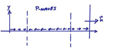
The uP particle
motion is in the direction of the ![]() vector
vector
For S waves (for simplicity, assuming A2 = 0)
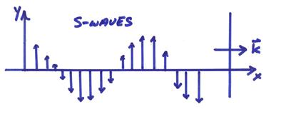
The uS particle
motion is perpendicular to ![]() in the plane of the wavefront
in the plane of the wavefront
Summary
Plane P waves – These produce longitudinal
displacement in the direction of propagation, have associated dilatation, and
propagate at the “P” velocity ![]() .
.
Plane S waves – These produce transverse motion perpendicular
to the direction of propagation, have associated rotation and shear strain, and
propagate at the S velocity ![]() .
.
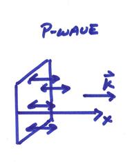
P-wave particle ground
motion parallel ![]()
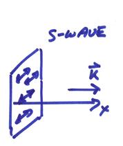
S-wave particle ground
motion perpendicular to direction of propagation ![]()
Finally, the flux rate of energy density of either plane P-waves or S-waves per unit time across a unit area normal to the direction of propagation is proportional to
![]()
Thus, the energy flux is proportional to the square of the
wave amplitude and also is proportional to ![]() where I is called the seismic wave impedance where V is equal to
where I is called the seismic wave impedance where V is equal to ![]() for P-waves and
for P-waves and ![]() for S-waves.
for S-waves.