EAS 557
Introduction to Seismology
Robert L. Nowack
Lecture 11
Elastodynamic Equation in an Unbounded Medium: Point Sources
The solution of the elastodynamic equation when a source term is included is now investigated. The elastodynamic equation can be written
![]()
Moving ![]() to the right side and
writing in vector notation
to the right side and
writing in vector notation
![]()
Now, using the vector identity ![]() , this can be written
, this can be written
![]() (1)
(1)
where ![]() and
and ![]() are the P and S speeds. If we let
are the P and S speeds. If we let ![]() be the input source
function and
be the input source
function and ![]() the resulting ground
displacement, then we can write
the resulting ground
displacement, then we can write
![]()
where T is the differential equation in equation (1), ![]() is the ground motion,
and
is the ground motion,
and ![]() is the source function. Using an input-output diagram,
is the source function. Using an input-output diagram,
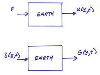
If the source function is a localized delta function in time
and space, then the output ground is written ![]() which is called the
Green’s function. This is similar to the
impulse response discussed earlier with respect to linear systems.
which is called the
Green’s function. This is similar to the
impulse response discussed earlier with respect to linear systems.
Let’s first
look at the simple wave equation for the scalar potential ![]()
 where
where ![]()
Then,

where ![]() . We will use Fourier
transforms to solve this. Let,
. We will use Fourier
transforms to solve this. Let,

and

This is a multi-dimensional, Fourier transform pair.
Note that similar to 1-D Fourier transforms, if
![]()
are Fourier transforms, then
![]()

![]()
![]()
Then, the scalar wave equation in the Fourier domain is ![]() . If
. If ![]() , then
, then ![]() . The solution to this
can be written,
. The solution to this
can be written,

Transforming back to the time and space domain, then

where
![]() = the Green’s function
for scalar wave equation
= the Green’s function
for scalar wave equation
For the case where ![]() is a constant, then
there are analytic solutions in each of the domains. The solution in different dimensions is given
below, where c is wave speed.
is a constant, then
there are analytic solutions in each of the domains. The solution in different dimensions is given
below, where c is wave speed.
|
|
|
|
|
|
|
|
|
|
|
|
|
for
|
|
|
|
|
|
|


The geometric spreading term in 1, 2 or 3 dimensions for the wave amplitude is
|
1-D |
2-D |
3-D |
|
|
|
|
In addition, the more complicated 2-D case has an amplitude
term proportional to ![]() in the
in the ![]() domain. In fact, Green’s functions for the scalar
wave equation in all even dimensional spaces are more complicated than Green’s
functions for odd dimensional spaces.
domain. In fact, Green’s functions for the scalar
wave equation in all even dimensional spaces are more complicated than Green’s
functions for odd dimensional spaces.
The basic idea is that if we know the Green’s function G(x,t), then for an arbitrary forcing function in time
![]()
then,
![]()
where ![]() is a time convolution
is a time convolution

In 3-D, the Green’s function is

and for a source time function f(t), then

For a general distributed source function in x and time, then

Let’s next look at the elasticdynamic Green’s function
 (2)
(2)
Let
![]()
which is a directed point force of position where ![]() is acting in the x1 direction and f(t)
is the source time function. The
multi-dimensional Fourier transform pair is
is acting in the x1 direction and f(t)
is the source time function. The
multi-dimensional Fourier transform pair is


If
![]()
then,
![]()

![]()
In the Fourier domain, equation (1) can be written
![]() (3)
(3)
Taking a dot product with k gives
![]()
Since ![]() , then
, then

Now using ![]() , equation (3) can be written
, equation (3) can be written

Then, using ![]() for the first term on
the right side
for the first term on
the right side
![]()

then

and
 (4)
(4)
Fourier transforming equation (4) back to the time and space domain gives
![]()
where

and c is either ![]() or
or ![]() .
.
Recall for the scalar wave equation in 3-D

Here,

If ![]() , where k is the
component in x1 direction,
then
, where k is the
component in x1 direction,
then ![]() , where i is the
component of displacement and 1 is the force direction. This is the Green’s function for the
elastodynamic equation.
, where i is the
component of displacement and 1 is the force direction. This is the Green’s function for the
elastodynamic equation.
For a point force in the x1 direction with time function f(t), then
![]()
then,
 for the field “P”
wave
for the field “P”
wave
 for the field “S”
wave
for the field “S”
wave
![]() near field terms of
combined P and S energy
near field terms of
combined P and S energy
where ![]() and
and ![]() are radiation patterns
and particle direction motion terms where
are radiation patterns
and particle direction motion terms where ![]() is the direction
cosine from the source to receiver.
is the direction
cosine from the source to receiver.
1) Properties of the far field P waves for single force
a) Attenuates as ![]() .
.
b) Propagates waveform f(t) at speed ![]() .
.
c) The displacement motion is parallel to the outward normal. uP has longitudinal motion since the particle motion is in the direction of propagation.
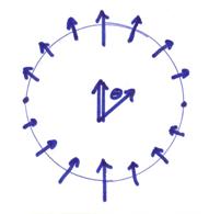
d) The directional radiation pattern motion is
proportional to ![]() where
where ![]() is shown in the figure
below.
is shown in the figure
below.
2) Properties of the far field S waves for single force
a) Attenuates as ![]() .
.
b) Propagates waveform f(t) at speed ![]() .
.
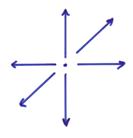
c) The direction of particle motion is perpendicular to the outward normal. Thus, uS has transverse motion
d) The directional radiation pattern is shown below.

The Green’s function for homogeneous elastic medium at one position with time for directed point force looks like
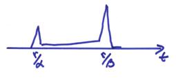
where the energy between ![]() and
and ![]() results from the near
field terms. Although the Green’s
function is for a single directed point force, in the Earth, forces usually
come in balanced combinations.
results from the near
field terms. Although the Green’s
function is for a single directed point force, in the Earth, forces usually
come in balanced combinations.
A superposition of directed point forces can be used to simulate realistic sources for homogeneous, as well as heterogeneous media. Then, for a heterogeneous media, the Green’s functions G may need to be computed numerically.
Examples of combinations of directed point forces include,
1) Explosion
6 directed point forces (3 dipoles)
2) Slip on small crack

A double set of couples
More complicated sources can be constructed by a superposition of Green’s function solutions.