EAS 557
Introduction to Seismology
Robert L. Nowack
Lecture 14A
Ray Theretical Methods
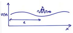
We will now investigate approximate solutions in heterogeneous media. Recall in a homogeneous medium, P and S plane waves of velocities can travel with the form


where ![]() . In a heterogeneous medium,
which is smooth and slowly varying, we will look for solutions of the form
. In a heterogeneous medium,
which is smooth and slowly varying, we will look for solutions of the form


where ![]() is the amplitude and
is the amplitude and ![]() is the eikonal or the
travel time. We want to put this into
the elastodynamic equation and solve for
is the eikonal or the
travel time. We want to put this into
the elastodynamic equation and solve for ![]() and
and ![]() , but first we would like to see what the restrictions of
using the “local plane wave” or “ray theory” solution is. These include,
, but first we would like to see what the restrictions of
using the “local plane wave” or “ray theory” solution is. These include,
1) The
frequency ![]() must be large, or
since
must be large, or
since
![]() ,
, ![]() , or
, or ![]()
this implies ![]() is small compared to
some scale in the medium. This can also
be considered as a short wavelength approximation.
is small compared to
some scale in the medium. This can also
be considered as a short wavelength approximation.
Ex) For a 1-D velocity structure with a
heterogeneity size “a”, then for ray
theory to be valid, ![]() must be much less than
“a”.
must be much less than
“a”.
2) Interfaces must be sufficiently smooth.
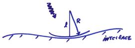
The radius of curvature of interface
l, must be much greater than the
wavelength, or ![]() . For this case, we
can use plane wave reflection and transmission coefficients, possibly corrected
for interface curvature.
. For this case, we
can use plane wave reflection and transmission coefficients, possibly corrected
for interface curvature.
3) The distance of propagation must not be too great.
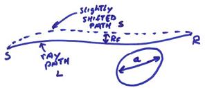
If a slightly shifted path has path length
![]() or less, then there
will be constructive interference for the energy traveling along these nearby paths
arriving at the receiver at R. Longer
paths will have greater travel times and might destructively interfere with energy
along the ray path. The zone of
constructive interference around the ray path is known as the first Fresnel zone.
The radius of the first Fresnel zone
about the ray is given by RF.
An idealized situation is shown below where the ray path has length L
and the slightly shifted path has length
or less, then there
will be constructive interference for the energy traveling along these nearby paths
arriving at the receiver at R. Longer
paths will have greater travel times and might destructively interfere with energy
along the ray path. The zone of
constructive interference around the ray path is known as the first Fresnel zone.
The radius of the first Fresnel zone
about the ray is given by RF.
An idealized situation is shown below where the ray path has length L
and the slightly shifted path has length ![]() .
.
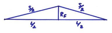
From the figure

or
![]()
Let
![]()
then,
![]() for
for ![]() .
.
Now,
![]() or
or ![]()
For ray methods to be valid, the heterogeneity scale “a” must be much greater than RF
or ![]() . Otherwise,
constructive interference won’t take place within the first Fresnel zone. This will put a limit on the propagation
distance to be
. Otherwise,
constructive interference won’t take place within the first Fresnel zone. This will put a limit on the propagation
distance to be
![]()
As an example, what would be the first Fresnel zone radius
for a ray reflected at the core mantle boundary (CMB) assuming a surface source
and receiver, f = 1 Hz and v = 10 km/sec? The wavelength ![]() will then be 10
km. The total path will be twice the
distance from the surface to the core mantle boundary, or L ~ 6000 km for a
vertical ray path. Then,
will then be 10
km. The total path will be twice the
distance from the surface to the core mantle boundary, or L ~ 6000 km for a
vertical ray path. Then,

This would be the radius of the zone on the CMB that would actively contribute and constructively interfere to give the reflected energy recorded at the surface, assuming the medium (i.e., the interface) is smooth over this length scale. If this is not the case, then Huygen’s principle needs to be used to estimate the diffracted energy from the rough boundary.
4) Ray methods break down at certain critical points where the amplitude gets large (infinite). These points are called caustics. There are certain modifications to the ray method that can be used to correct this restriction using high frequency ray methods. These modified methods include
1) The Maslov method
2) The Gaussian Beam seismograms
But, these more advanced methods won’t be discussed further here.
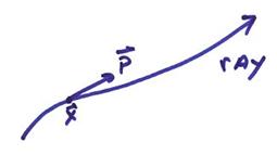
Let’s look now at seismic energy along rays. The travel time along a ray can be written as
where
![]() : The velocity along
the ray at position
: The velocity along
the ray at position ![]()
![]() : The starting point
of the ray
: The starting point
of the ray
![]() : The ending point of
the ray
: The ending point of
the ray
![]() : The travel time
(eikonal) along the ray
: The travel time
(eikonal) along the ray
s: The path length along the ray

A general way of specifying a ray is
via Fermat’s principle, which states that the travel time ![]() is a mininum or a maximum
(an extremum) along the actual ray path.
This can be written as
is a mininum or a maximum
(an extremum) along the actual ray path.
This can be written as ![]() for a small change in
the path. Thus, nature is economical and
picks out the path that the seismic energy will travel along that provides a
minimum (an extremum) travel time.
for a small change in
the path. Thus, nature is economical and
picks out the path that the seismic energy will travel along that provides a
minimum (an extremum) travel time.
We can derive the ray tracing equations from Fermat’s principle. Let
where we have inserted a term in brackets in the integral
that is formally equal to 1 since ![]() . The integrand can be
written as
. The integrand can be
written as
![]() i =
1, 3
i =
1, 3
where ![]() is
is ![]() . The travel time
integral is then
. The travel time
integral is then
Fermat’s principle says a small
change in the travel time about a ray will be zero (![]() is an extremum about a valid ray for a small change in path). Thus,
is an extremum about a valid ray for a small change in path). Thus,

where ![]() is small variation in the
travel time. This can be written as
is small variation in the
travel time. This can be written as
 summation on i (i
= 1,3)
summation on i (i
= 1,3)
Now,
then,
Using integration by parts for the
second term where ![]() , and letting
, and letting
![]() and
and ![]()
then,
where the first term ![]() is zero for fixed end
points. Now,
is zero for fixed end
points. Now,
For this to be true for an arbitrary path, then the term in brackets must be zero giving

These are called Euler’s equations, where i = 1,3.
Since

then,
where ![]() is 1. For the Euler equations, this results in
is 1. For the Euler equations, this results in
 i = 1,3
Now define ![]() where
where  is the slowness vector
tangent to the ray, then
is the slowness vector
tangent to the ray, then
![]()
![]() i = 1,3
i = 1,3
These are called the ray equations in an isotropic, heterogeneous medium which solve for the position (x) along the ray and the slowness vector p tangent to the ray at each point.
Now, several examples will be given for rays in different types of media.
Ex) For
a constant velocity medium, v =
constant, then ![]() .
.
Thus, p1, p2, p3 are equal to constants along the whole ray. Ray will then be straight lines from the source.
Ex) For
a vertically varying medium, with ![]() , then
, then ![]() .
.
Thus, p1, p2 will be constants along the ray. The horizontal slowness will then be conserved
along the entire ray. For a ray in the (x1,x3) plane, ![]() constant where
constant where ![]() is the angle of the
ray from the vertical. Special ray
equations are derived later for vertically and radially varying media.
is the angle of the
ray from the vertical. Special ray
equations are derived later for vertically and radially varying media.
Ex) For a horizontal interface between two constant velocity half spaces, then
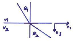
for a ray in the (x1,x3) plane, ![]() . This is Snell’s
law where p1 = constant
for both ray segments.
. This is Snell’s
law where p1 = constant
for both ray segments.
Ex) For media with laterally and vertically varying velocities, than a computer program must be used to solve the ray equations.
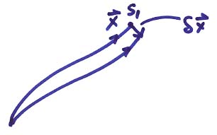
After the rays are
determined, the travel times can be computed along the ray as  .
.
Assume that
the path satisfies the ray equations and consider a perturbation of the endpoint
s1
Now,
 i = 1,3
For a valid ray path, the integral is zero and
![]()
Recall that
![]()
then,
![]()
where p1
can be identified as ![]() and similarly for p2 and p3. Thus,
and similarly for p2 and p3. Thus,
![]() i = 1,3
i = 1,3
which is the grad vector of the time field in the direction of the ray. Then,

This is called the Eikonal equation. For any perturbation vector ![]() parallel to the wavefront,
then
parallel to the wavefront,
then ![]() and
and
![]()
or
![]()
Thus, for an isotropic medium, ![]() is perpendicular to the
wavefront.
is perpendicular to the
wavefront.
We therefore have three ways to specify ray paths in a heterogeneous medium,
1) Fermat’s principle
2) The ray equations
3) The Eikonal equation
In order to
investigate the equation of motion, we will first look at the P wave potential ![]() which solves the
simple wave equation
which solves the
simple wave equation

Since plane waves are solutions to this equation for v = constant, we will look for “local plane wave” solutions in the high frequency limit for heterogeneous media. A trial solution can be written

which is an “asymptotic ray series”. An asymptotic series is valid for some parameter
sufficiently large or small. For the ray
series, ![]() is assumed to be large
or
is assumed to be large
or ![]() is assumed to be small
(with respect to some scales of the medium).
Now substitute the trial solution into the wave equation. This results in
is assumed to be small
(with respect to some scales of the medium).
Now substitute the trial solution into the wave equation. This results in

![]()
![]()
The idea is to set each of the brackets to zero separately
for the case where ![]() is large. If
is large. If ![]() were not large,
we would have to solve all brackets at once – as in the original equation. Setting the
were not large,
we would have to solve all brackets at once – as in the original equation. Setting the ![]() term to zero results
in
term to zero results
in
![]()
which is the Eikonal equation derived earlier from the ray equations. The zero-th order solution is then
![]()
Next, set the ![]() term to zero resulting
in
term to zero resulting
in ![]() . This is called the
transport equation.
. This is called the
transport equation.
From the transport equation
![]()
where J(s) is the geometric spreading which can be determined from the geometry of the rays obtained from the zero-th order term. The geometric spreading depends on the type of source and the velocity variations along the path and can be obtained from the rays by solving the “dynamic ray equations”. For example, for a point source in a 3-D homogeneous medium, the geometrical spreading is related to the distance from the source squared. The first order ray solution to the wave equation is
![]()
where ![]() is assumed to be large.
is assumed to be large.
In order to calculate ray theoretical seismogram in a variable velocity medium
1) Compute rays by solving the ray equations.
2) Compute the travel time for rays from the source to the receivers.
3) Compute the geometric spreading J along the rays using the dynamic ray equations.
4)
Construct ![]() .
.
5) Convolve with source time function.
For example, a computer program SEIS88 performs these steps for a heterogeneous 2-D medium.
The complete, isotropic elastodynamic equation can be written as

where

A trial ray series solution can then be written as

where it is assumed that ![]() is large. Putting this trial solution into the elastodynamic
equation, the
is large. Putting this trial solution into the elastodynamic
equation, the ![]() term is
term is

where
 and
and 
This is zero if either
1)
![]()
or
2)
![]()
Thus, in the high frequency approximation, two waves can
propagate (P and S) in an isotropic, heterogeneous medium. Also, it can be found that the particle
motion for a high frequency P-wave is in the direction of the ray and for a
high frequency S-wave is perpendicular to the ray along the wavefront. Recall in the homogeneous case, velocities ![]() and
and ![]() are constant and the
elastodynamic equation can be strictly separated into two wave types (P and S). For the heterogeneous case in the high
frequency limit, this is still approximately true.
are constant and the
elastodynamic equation can be strictly separated into two wave types (P and S). For the heterogeneous case in the high
frequency limit, this is still approximately true.