EAS 557
Introduction to Seismology
Robert L. Nowack
Lecture 14C
Ray Method in a Layered Flat Earth
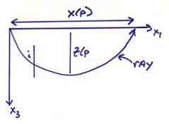
For a horizontally layered media, the ray equations reduce to integrals for distance and travel-time given the ray parameter p. We will again investigate a common-shot gather with the shot at the origin and receivers located along the x3 = 0 plane.
The distance and travel time integrals can be written
where Z(p) is the
maximum depth of the ray. Since ![]() is a constant along
the ray for a layered medium, then
is a constant along
the ray for a layered medium, then ![]() at the bottoming depth
where the tangent of the ray is horizontal.
at the bottoming depth
where the tangent of the ray is horizontal.
We want to derive another useful formula for p. Consider a plane wave incident at the receiver
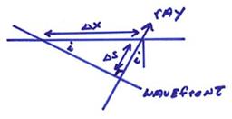
From the figure above during the time ![]() , the wavefront will have moved
, the wavefront will have moved ![]() . So, the velocity
along the ray is
. So, the velocity
along the ray is ![]() . The horizontal
apparent velocity in the x direction is
. The horizontal
apparent velocity in the x direction is
![]() . Then,
. Then,
![]()
or
![]()
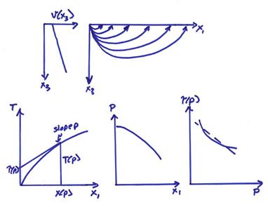
Thus, p can be measured as the slope of the travel time curve for receivers along the surface.
Let’s now go back to the travel-time integral
We now use integration by parts ![]() to find
to find
or

Now, we can define a new variable  , then
 ![]() can be written
can be written
![]()
This defines a line in [T,X] space with slope p and intercept ![]() .
.
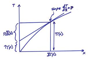
![]() can then be decomposed
into pX(p) and
can then be decomposed
into pX(p) and ![]() , where pX(p) is the time corresponding to
horizontal propagation with velocity vx
= p-1 for the wave to
travel a distance X(p).
, where pX(p) is the time corresponding to
horizontal propagation with velocity vx
= p-1 for the wave to
travel a distance X(p).
The
function ![]() can be written
can be written
![]()
Substituting the integrals for ![]() and
and ![]() , this becomes
, this becomes
or
where the integrand is just equal to p3 which is one over the apparent velocity in the x3 direction. Thus, ![]() is the time corresponding
to the vertical travel distance, Z(p),
and the integral of the vertical slowness along the ray path. Thus for
is the time corresponding
to the vertical travel distance, Z(p),
and the integral of the vertical slowness along the ray path. Thus for
![]()
![]() is the time component
associated with the horizontal travel distance
is the time component
associated with the horizontal travel distance ![]() and
and ![]() is the time component associated
with the two-way vertical travel distance.
is the time component associated
with the two-way vertical travel distance.
Now, recall
then,
![]()
Since ![]() is a positive
distance, the slope of
is a positive
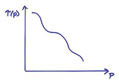
distance, the slope of ![]() is always negative. Thus,
is always negative. Thus, ![]() is a monotonically
decreasing function of p as shown
below.
is a monotonically
decreasing function of p as shown
below.
The following formulas then summarize the travel time as a function of ray parameter p.
![]()
and
![]()
and
![]()
We now give several examples of these functions.
1) A linear T(x) curve. This will result
from a wave traveling horizontally in a constant velocity medium ![]() . Then, the following
graphs can be drawn.
. Then, the following
graphs can be drawn.
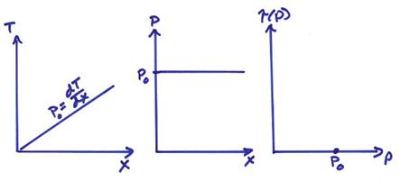
In the ![]() graph, a horizontally
traveling wave plots as a point.
graph, a horizontally
traveling wave plots as a point.
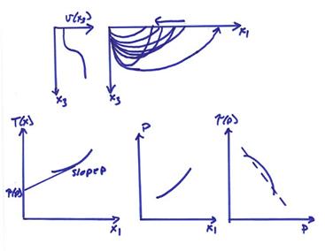
2) A “normal branch” of travel time curve. For this case, X(p) is increasing with decreasing p.
Now,
since ![]() ,
then for this case
,
then for this case

Also
![]()
where
![]() is a decreasing
function of p. Then,
is a decreasing
function of p. Then,

Thus,
 for a normal branch of
the travel time curve.
for a normal branch of
the travel time curve.
3) A “reverse branch” of the travel time
curve. For this case, ![]() is decreasing with
decreasing p. This would occur for a rapid increase in the
velocity with depth.
is decreasing with
decreasing p. This would occur for a rapid increase in the
velocity with depth.
Again,
![]() and for this case
and for this case

Also,
![]()
where
![]() is the decreasing
function of p. Thus,
is the decreasing
function of p. Thus,

for a reverse branch of the travel time curve.
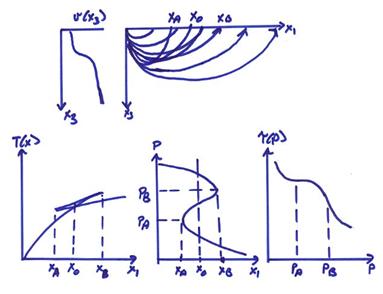
Ex) A continuous velocity increase with depth
with a zone of rapid velocity increase.
For this case, the travel times will initially be a normal branch
followed by a reverse branch and then returning to a normal branch. This will result in a triplicated T(X)
curve. The ![]() curve has the effect
of unwrapping the triplication.
curve has the effect
of unwrapping the triplication.
Again, ![]() and
and  , then
![]() for the reverse branch,
and
for the reverse branch,
and ![]() for the normal branches.
for the normal branches.
Also,
![]()
Thus, ![]() is a decreasing
function of p. Then,
is a decreasing
function of p. Then,
 for the normal branches,
and
for the normal branches,
and  for the reverse branch.
The ![]() function can be
plotted with
function can be
plotted with ![]() going down to better represent
a two-way vertical travel-time which we want to relate to depth. p-1
is the apparent horizontal velocity and is also the actual velocity at the
bottoming point of the ray.
going down to better represent
a two-way vertical travel-time which we want to relate to depth. p-1
is the apparent horizontal velocity and is also the actual velocity at the
bottoming point of the ray.
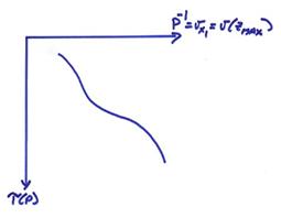
This looks similar to the original v(x3) plot
except plotted in ![]() instead of depth. In fact, we can use the
instead of depth. In fact, we can use the ![]() curve to invert for v(x3)
by converting the
curve to invert for v(x3)
by converting the ![]() axis to a depth axis
by a downward continuation inversion process.
axis to a depth axis
by a downward continuation inversion process.
Ex) A layer over half space. For this case, we have both pre-critical and
post-critical reflections from the interface, in addition to a refraction from
the interface. The different curves T(x) and ![]() are shown below.
are shown below.
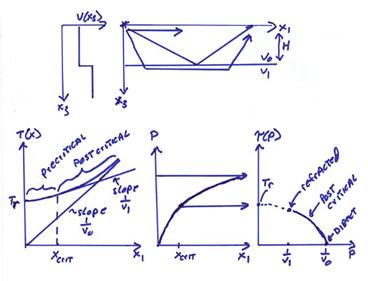
If we have just first arrivals, there would be an infinite
number of ![]() curves that would pass
through the two points associated with the direct and refracted first
arrivals. The later reflected arrivals
are needed to constrain the complete
curves that would pass
through the two points associated with the direct and refracted first
arrivals. The later reflected arrivals
are needed to constrain the complete ![]() curve and also
uniquely invert for the velocity with depth.
curve and also
uniquely invert for the velocity with depth.
Ex) A velocity profile with a low velocity zone. For this case, we have a shadow formed in distance resulting from rays traveling through the low velocity zone.
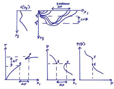
This will result in a nonuniqueness in inverting for v(x3)
since no rays bottom inside the LVZ.
Nonetheless, we can get upper bounds on thickness of the LVZ by the observation
of ![]() and
and ![]() from the travel time
curve.
from the travel time
curve.
Ex) An arbitrary point on a seismic trace from a
seismic record section. For this case,
each point on a seismogram has a specific distance X, but any line of slope p can fit through it. Thus, a point on a seismic record section
will plot as a line in ![]() .
.
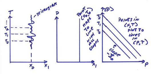
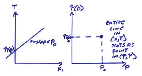
Thus, a seismogram in T(x)
plots as a series of lines with slope –X(p)
and intercepts Ti in ![]() . In contrast, a line
in T(X) with slope p0 plots
as point in
. In contrast, a line
in T(X) with slope p0 plots
as point in ![]() as shown below.
as shown below.
![]() can be constructed
point by point by slant stacking a seismic record section. An example of this is shown below.
can be constructed
point by point by slant stacking a seismic record section. An example of this is shown below.
Finally, if
we are given ![]() or X(p), we can use this function to uniquely
reconstruct v(x3) (assuming no LVZ’s are present). This was first done by Herglotz (1907) and Wiechert
(1910). Wiechert was the director of the
first geophysical observatory located in
or X(p), we can use this function to uniquely
reconstruct v(x3) (assuming no LVZ’s are present). This was first done by Herglotz (1907) and Wiechert
(1910). Wiechert was the director of the
first geophysical observatory located in
We will investigate X(p) which can be written as
 (*)
(*)
The Abel transform pair can be written as
and
provided ![]() is continuous, and has
finite derivatives.
is continuous, and has
finite derivatives.
We can then rewrite equation (*) as
Let
![]()
![]()
![]()
![]()
then from the Abel transform pair,
and,
Since ![]() , from
, from ![]() , then also
, then also
Thus, the depth to a given velocity v can be gotten from either X(p)
data or ![]() data, but no LVZ’s are
allowed for this to work exactly. Thus,
X(p) and
data, but no LVZ’s are
allowed for this to work exactly. Thus,
X(p) and ![]() must be continuous.
must be continuous.
We next show several examples of velocity depth curves and corresponding travel time functions. The figure below shows the average radial velocity structure for the Earth. Two models are shown, the Jeffreys-Bullen model and the IASP91 model.
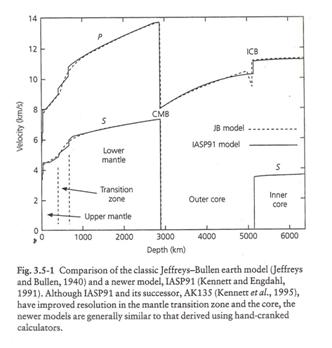
(from Stein and Wysession, 2003)
The predicted travel times from the IASP91 model are shown below for a surface focus earthquake and an earthquake with a 600 km focal depth.
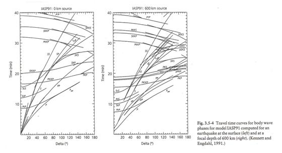
(from Stein and Wysession, 2003)
The figure below shows the notation for different ray paths in the Earth.
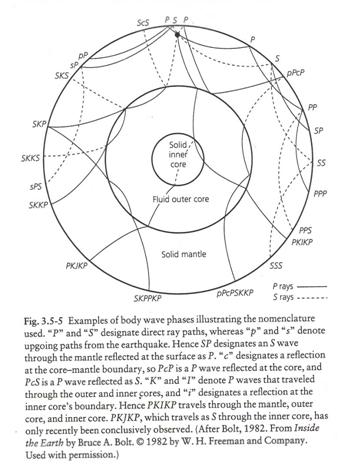
(from Stein and Wysession, 2003)
The naming convention for different ray paths are also given in the table.
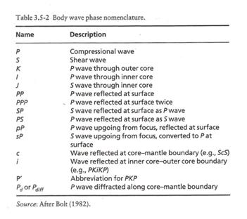
(from Stein and Wysession, 2003)
The figure below shows an example of a typical long period seismogram with the phases marked. The ray paths in the upper mantle are also shown. On the right is a picture of travel picks for a data set of 57,655 observed travel-times from 104 sources with the theoretical travel-times from IASP91 also shown.
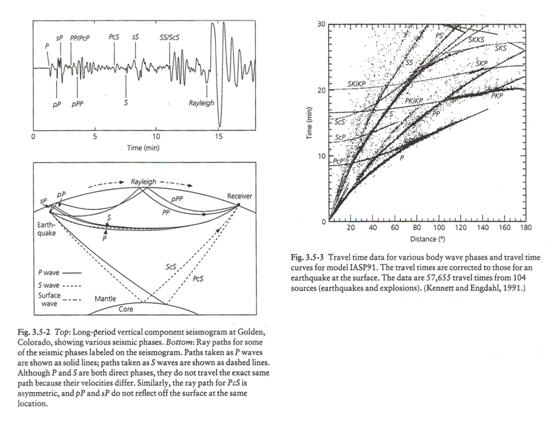
(from Stein and Wysession, 2003)
The figure below shows a ray trace through a crustal model. The upper plot shows seismic data with the predicted travel times computed from the ray trace in the model in the lower plot.
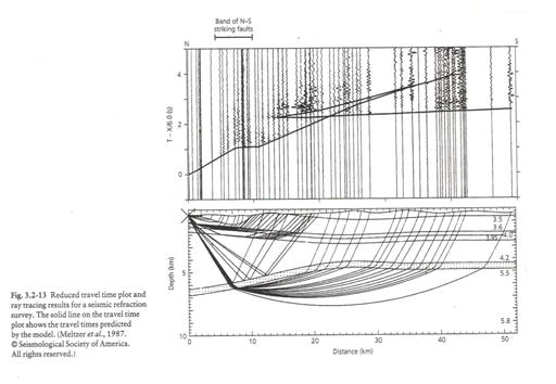
(from Stein and Wysession, 2003)
The figure below shows a ray trace through the upper mantle. The complexities of the rays result from velocity increases in the upper mantle at depths near 410 km and 660 km.
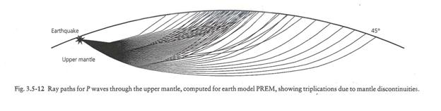
(from Stein and Wysession, 2003)
The figure below shows predicted mineral assemblages as a function of depth in an upper mantle of a pyrolite composition (from Ringwood, 1979).
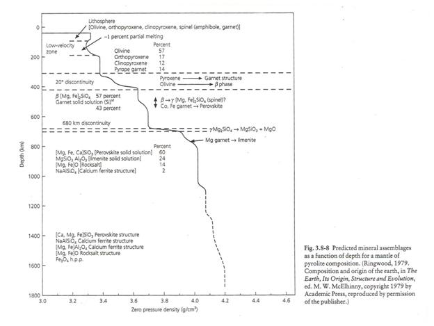
(from Stein and Wysession, 2003)
The figure below shows ray tracing in the Earth’s core and mantle using the PREM Earth model.
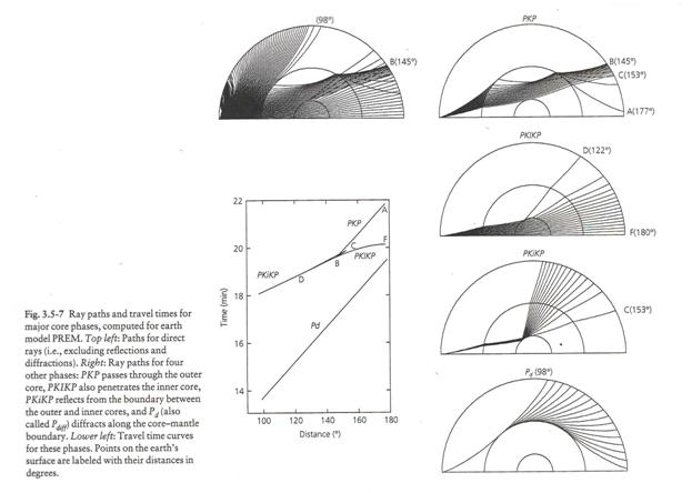
(from Stein and Wysession, 2003)
The figure below shows synthetic seismograms for an upper mantle model derived from earthquake data in the Western Pacific recorded at different distances from the Taiwan Seismic Array. The synthetic seismic data shows two upper mantle triplications in a reduced travel time format for T – X/10.
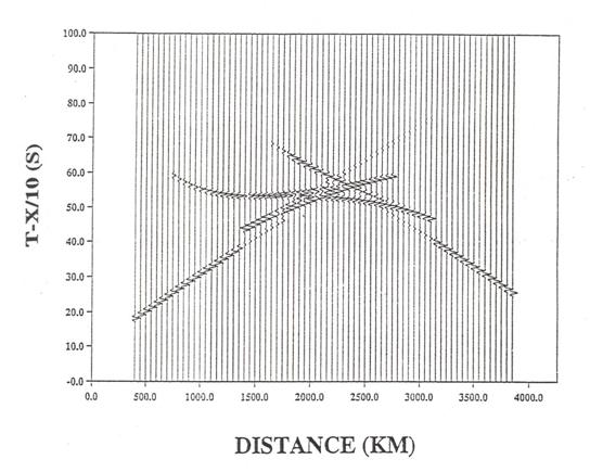
(from Nowack et al., 1999)
The figure
below shows the result of slant stacking the synthetic seismic data in the
previous figure. The data is plotted in p-1 = v with ![]() going down.
going down.
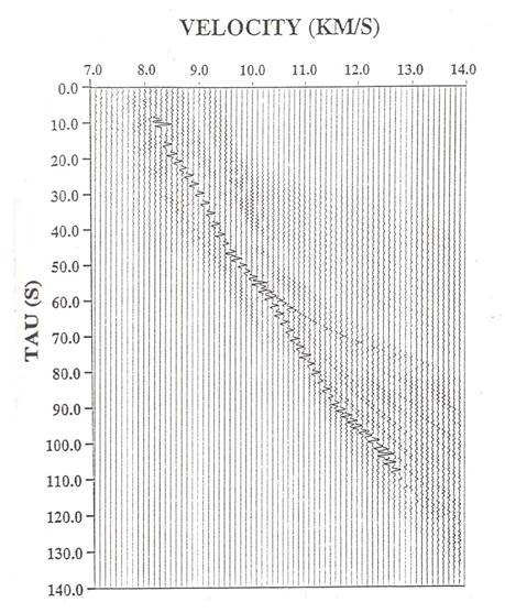
(from Nowack et al., 1999)
The figure below shows the results of imaging the slant stacked data. This gives an estimate of the velocity depth function in Earth flattened coordinates. The true model in Earth flattened coordinates is shown by the solid line.
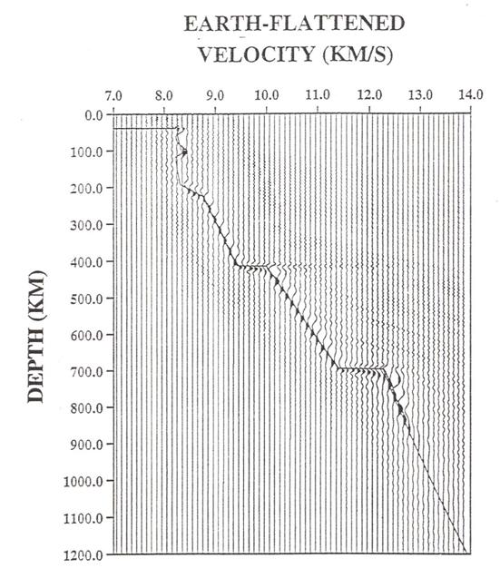
(from Nowack et al., 1999)