EAS 557
Introduction to Seismology
Robert L. Nowack
Lecture 15A
Seismic Surface Waves
We now investigate seismic surface waves which have the following properties.
1) Surface waves propagate parallel to the Earth’s surface.
2) Amplitude as a function of depth is stationary with horizontal distance (apart from spreading and anelastic viscoelastic attenuation). The amplitude decay from geometric spreading for different waves is
surface
waves ![]() (cylindrical
spreading)
(cylindrical
spreading)
body
waves ![]() (spherical
spreading)
(spherical
spreading)
refracted
head waves ![]()
Thus, at long ranges, surface waves will be larger in amplitude than the body waves.
3) Long period surface waves give information about earth structure as well as the source mechanism.
4) In seismology, the most important interface is the Earth’s free surface.
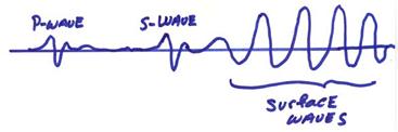
5) Except for first arriving P and S waves, surface waves will be the most prominent ground disturbance seen on seismograms. Also, their character is very different than body waves.
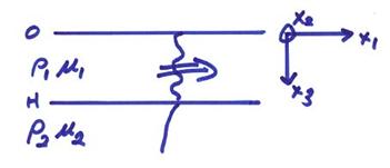
As a first example, we’ll look at the antiplane (SH) case for a layer over a half space. The antiplane guided waves are called Love waves. Consider, the elastodynamic equation with fi = 0. For an isotropic solid

and

Consider an SH wave traveling in the x1 direction, but with particle motion in the x2 direction.

Substituting this into the elastodyamic equation then,

For SH particle motion in a layer
over a half space with ![]() , then a horizontally propagating wave, called a Love wave,
can exist,
, then a horizontally propagating wave, called a Love wave,
can exist,
where ![]() and
and ![]() . Within the layer,
. Within the layer,

In the halfspace,

Now, we will use the trial solution
![]()
The boundary conditions of the problem are
![]() at
the interface on plane x3
= H
at
the interface on plane x3
= H
![]() at
the interface on plane x3
= H
at
the interface on plane x3
= H
![]() on
the free surface
on
the free surface
What kind of solution are we looking for?
1) We want surface waves, i.e., waves whose displacements are confined, “close” to the free surface x3 = 0 and don’t increase in amplitude with increasing depth.
2) We want a wave whose horizontal velocity, ![]() is the same for all
depths x3. (In particular, the horizontal speed should
be the same for the layer and the half space.)
is the same for all
depths x3. (In particular, the horizontal speed should
be the same for the layer and the half space.)
3) The phase velocity ![]() could possibly be
frequency dependent.
could possibly be
frequency dependent.
This is not the same problem as plane waves incident on a
boundary at some angle ![]() . We are trying to
find a solution to the equation of motion which is a wave of a different kind with
the properties listed above.
. We are trying to
find a solution to the equation of motion which is a wave of a different kind with
the properties listed above.
We seek a
solution propagating along the x1
axis with horizontal phase velocity ![]() and time dependence
and time dependence ![]() , where
, where ![]() and
and ![]() . Use the solution
form
. Use the solution
form ![]() for the layer and a
similar form for the half space and put these into the equation of motion. Then
for the layer and a
similar form for the half space and put these into the equation of motion. Then

or,

for the layer and a similar equation for the half space. A solution for h(x3) can be written
![]() in
the layer for
in
the layer for ![]()
![]() in
the half space for x3 >
H
in
the half space for x3 >
H
where
 for
0 < x3 < H
for
0 < x3 < H
 for
x3 > H
for
x3 > H
We now have unknowns ![]() .
.
We now apply the boundary conditions to solve for the unknowns.
1) First, we will assume that there are no
sources at ![]() and thus no up-going
waves in the lower half space. Thus,
and thus no up-going
waves in the lower half space. Thus, ![]() in the lower half
space.
in the lower half
space.
2) If ![]() or
or ![]() , then
, then  and
and ![]() . We thus want an evanescent
wave in the half space, i.e., an exponentially decreasing function with depth
in the halfspace.
. We thus want an evanescent
wave in the half space, i.e., an exponentially decreasing function with depth
in the halfspace.
3) At the free surface, ![]() at x3 = 0. Then,
at x3 = 0. Then,
![]()
This gives
![]()
We are then down to three unknowns ![]()
4) We must now satisfy continuity of displacement and traction at the interface x3 = H.
For displacement ![]()
For traction ![]()
Now, recall
![]()
and
![]()
Now, the above two equations can be written
![]()
![]()
then,
This gives two equations for ![]() if we know k1. The equality between the right two terms gives
an equation
if we know k1. The equality between the right two terms gives
an equation ![]() . This is called a dispersion
relation for
. This is called a dispersion
relation for ![]() . Thus,
. Thus,
where the vertical wavenumbers for the layer and half space can be written.


![]() is
an implicit equation to find
is
an implicit equation to find ![]() or
or ![]() . The solution is
called an eigenvalue for a given frequency
. The solution is
called an eigenvalue for a given frequency
![]() . Writing this in
terms of
. Writing this in
terms of ![]() gives
gives

where ![]() results in an evanescent
wave in the lower half space.
results in an evanescent
wave in the lower half space.
We will use
a graphical method to solve this for ![]() . For
. For
![]() , then there are real roots to
, then there are real roots to
![]()
where


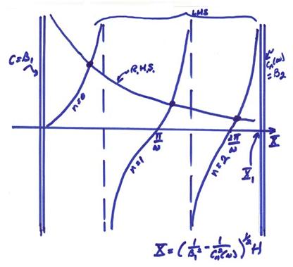
At X = 0, ![]() . For
. For
![]() ,
, ![]() , and
, and

The following comments can be made.
1) Real roots are limited to lie between ![]() .
.
2) For any given frequency ![]() , there will be multiple roots (but only a countable number
of them).
, there will be multiple roots (but only a countable number
of them).
3) For ![]() , the tangent curves will expand giving only the n = 0 curve between the
, the tangent curves will expand giving only the n = 0 curve between the ![]() and
and ![]() lines.
lines.
4) For slightly larger ![]() , the n = 1 tangent
curve will enter the real region from the right. It enters when
, the n = 1 tangent
curve will enter the real region from the right. It enters when ![]() is such that
is such that

5) For larger ![]() , more of the tan curves enter from the right. The nth curve enters when
, more of the tan curves enter from the right. The nth curve enters when

This is called the cutoff for the nth
higher mode. The nth higher
mode can only propagate for ![]() .
.
Ex)
The continental crust beneath
![]() = 3.5 km/sec
= 3.5 km/sec ![]() = 4.5 km/sec
= 4.5 km/sec
then,
![]() where
where ![]() = 0.08 Hz
= 0.08 Hz
or the period of
the cutoff for the 1st higher mode is ![]() = 13 sec =
= 13 sec = ![]() . Thus, for this velocity
structure, only the n = 0 fundamental
mode Love wave can propagate for T
> 13 sec (or
. Thus, for this velocity
structure, only the n = 0 fundamental
mode Love wave can propagate for T
> 13 sec (or ![]() cycles/sec).
cycles/sec).
6) At each mode’s cutoff frequency, then ![]() .
.
7) As ![]() ,
, ![]() for all modes and a
large number of them can propagate.
for all modes and a
large number of them can propagate.
A graph of the horizontal velocities as a function of frequency is shown below. (This is often also plotted as a function of period.)
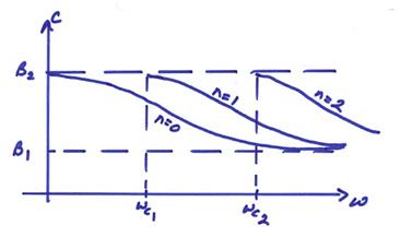
The
change of ![]() with
with ![]() is called the dispersion
curve for a given mode number n.
is called the dispersion
curve for a given mode number n.
Now with
the eigenvalues derived ![]() or
or ![]() ) which satisfy the dispersion relation, the corresponding
vertical eigenfunction h(x3) can be
found as
) which satisfy the dispersion relation, the corresponding
vertical eigenfunction h(x3) can be
found as
where

The vertical eigenfunction is a sinusoidal standing wave in x3 in the layer and exponentially decreasing in the lower half space. The first three eigenfunctions for a frequency near the cutoff frequency and at a larger frequency are shown below.
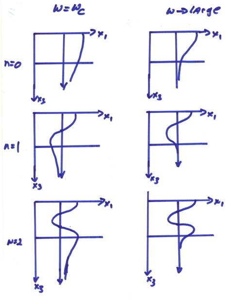
Different mode numbers correspond to a different number of zero crossings in the layer. Also, each mode for each frequency travels at a different horizontal speed.
If a source is at one of these nodal depths, then the source will not be very efficient in generating that mode or vertical eigenfunction for that frequency.
For an actual source, we must superpose all allowable modes to satisfy the given source condition.
For more
layers than one, we must use a computer program to solve the dispersion
relation for k1 or ![]() , as well as to find the vertical eigenfunctions. The steps include:
, as well as to find the vertical eigenfunctions. The steps include:
1) Solve the dispersion relation for ![]() for a given
for a given ![]() .
.
2) Solve for the vertical eigenfunction
![]() for each
for each ![]() for a given
for a given ![]() .
.
3) Superpose the different eigenfunctions to satisfy a source condition for each frequency.
4) Superpose all frequencies for the source excitation.
5) If this is done correctly, this will simulate the surface wave contributions to the seismic signal.
Next, we will look at the P-SV case for in plane particle motion.