EAS 557
Introduction to Seismology
Robert L. Nowack
Lecture 16
Free Oscillations
We have so far considered waves generated by earthquakes as propagating disturbances in infinitely extended spaces (i.e., whole spaces, half spaces with a free surface, a layered half space, etc.). But, the Earth is a bounded region; to first order a sphere.
In such bounded systems, we can consider the total motion to be made up of a sum of vibrations or “normal modes of free oscillations”. Thus, a seismogram recording motion from a distant earthquake can be thought of as a series of traveling waves P and S, etc. or as a sum of “standing waves” or free oscillations adding together at a given location x and time t to produce the observed seismogram with all of the “body waves” and “surface waves” included.
So, what is a “normal mode” or free oscillation?
1) It satisfies the elastodynamic equation of motion
2) It satisfies all the boundary conditions
3) It can exist without a source
For a finite body there will be a discrete set of modes
(possibly large, but countable in number).
Thus, the solution can be written as a sum of modes as ![]() modes.
modes.
Ex) Vibrations on a fixed string.
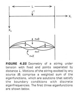
For a string then, we can write the equation of motion as
 for
for
![]() and
and ![]()
The speed is ![]() , where T is the tension of string and
, where T is the tension of string and ![]() is the density.
is the density.
The boundary conditions are ![]() . The initial
conditions are
. The initial
conditions are ![]() and
and ![]() for
for ![]() . Use separation of
variables (S.O.V.) to solve this, let
. Use separation of
variables (S.O.V.) to solve this, let
![]()
Then
![]()
where k is some constant. Then,
![]()
This is an eigenvalue problem with
![]()
The solution can be written as
![]()
where from the boundary conditions
![]()
![]()
Then,
![]() or
or ![]() , for
, for ![]()
The ![]() are called the eigenvalues and
are called the eigenvalues and ![]() are called the eigenfunctions.
are called the eigenfunctions.
Solving for
![]() then
then
![]()
![]()
The ![]() are called the
normal modes (or free oscillations) for the string. It is a global solution on the domain
are called the
normal modes (or free oscillations) for the string. It is a global solution on the domain ![]() .
.
Now we must
superimpose normal modes to satisfy the initial conditions ![]() and
and ![]() . Then,
. Then, ![]() is a “standing wave”
with nodal points at
is a “standing wave”
with nodal points at ![]() (
(![]() ). These normal modes
can also be expressed as a sum of propagating waves of the form
). These normal modes
can also be expressed as a sum of propagating waves of the form
![]() . Recall that
. Recall that
![]()
and
![]()
then,
![]()
![]()
Thus, a standing wave can be written as a combination of left and right propagating traveling waves. This contrasting view of standing waves or modes as reverberating traveling waves is a fundamental theme coming up again and again in seismology. Thus, in terms of normal modes the resulting motion can be written as a sum of normal modes satisfying the initial conditions
![]()
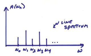
The frequency of each mode is ![]() and these form a
discrete spectrum. The contribution from
each frequency may
be represented by an amplitude
and these form a
discrete spectrum. The contribution from
each frequency may
be represented by an amplitude
![]()
thus,
Strictly speaking, we use the term spectrum for something we
can Fourier analyze (i.e., the displacement history at a point ![]() on the string
on the string ![]() ), then
), then
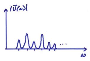
Because of friction on the string, we get a continuous spectrum instead of just a line spectrum. Each peak gives us a normal mode frequency.
Well, you might say that a vibrating string doesn’t look much like the Earth. However, all that we’ve talked about carries over to the Earth as a much more complex boundary value problem.
Free Oscillations of
the Earth
Recall the elastodynamic equation
![]() with
with
![]()
where ![]() is the body force due
to gravity. What we are faced with is
the solution to this equation subject to vanishing tractions on the Earth’s
surface and continuity of displacements and tractions at any internal boundary. Also, we must include the body forces due to
gravity here. This makes a difference
for periods T > 200 sec.
is the body force due
to gravity. What we are faced with is
the solution to this equation subject to vanishing tractions on the Earth’s
surface and continuity of displacements and tractions at any internal boundary. Also, we must include the body forces due to
gravity here. This makes a difference
for periods T > 200 sec.
Cartesian coordinates are inappropriate for low frequency waves in the spherical Earth. Thus, we must introduce spherical coordinates.
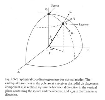
(from Stein and Wysession, 2003)
For example, let’s look at the free oscillations of a homogeneous liquid sphere where

where P is the pressure subject to ![]() on the surface
on the surface ![]() . Then, in spherical
coordinates
. Then, in spherical
coordinates


In exactly the same way as for the string, we use separation of variables and look for a solution of the form
![]()
and for each of the terms,
1) ![]()
2) ![]() where l and m are integers
where l and m are integers ![]() and
and ![]() are called the associated
Legendre functions, i.e.
are called the associated
Legendre functions, i.e.
3 ![]() gives the amplitude as a function
of depth in the Earth. This is similar
to the eigenfunction in depth for surface waves and
for a spherical Earth is written in terms of spherical Bessel functions.
gives the amplitude as a function
of depth in the Earth. This is similar
to the eigenfunction in depth for surface waves and
for a spherical Earth is written in terms of spherical Bessel functions.
The eigenvalues for
this problem can be written ![]() where n is the overtone number and l is the spherical Bessel function
order. n is also equal to the number of
zero crossings in depth.
where n is the overtone number and l is the spherical Bessel function
order. n is also equal to the number of
zero crossings in depth.
Elastic Earth –
Vector Spherical Harmonics
As in the case for surface waves, for a spherical Earth with elastic properties that vary only as a function depth, then the motions separate two types of motion
1) Toroidal motions have
particle displacements with ![]() and
and ![]() . Toroidal
motions have only horizontal motion and are like “SH” Love waves. They are written as
. Toroidal
motions have only horizontal motion and are like “SH” Love waves. They are written as ![]() .
.
2) Spheroidal motions
have particle displacements with ![]() . Spheroidal
motions include both vertical and horizontal motion like “P-SV” Rayleigh waves and are written as
. Spheroidal
motions include both vertical and horizontal motion like “P-SV” Rayleigh waves and are written as ![]() .
.
For both cases, ![]() resulting in
resulting in ![]() values. Toroidal and spheriodal oscillations have their own sets of normal mode
frequencies which depend on the constants n,
m, l determined from the boundary conditions.
values. Toroidal and spheriodal oscillations have their own sets of normal mode
frequencies which depend on the constants n,
m, l determined from the boundary conditions.
If the effect
of the Earth’s rotation is neglected, then the eigenvalues
![]() are independent of m.
The (2l + 1) degeneracy then
results in just one Fourier amplitude peak.
However, with rotation included this degeneracy breaks down. This is similar to rotational splitting of
atomic spectrum lines due to a magnetic field.
are independent of m.
The (2l + 1) degeneracy then
results in just one Fourier amplitude peak.
However, with rotation included this degeneracy breaks down. This is similar to rotational splitting of
atomic spectrum lines due to a magnetic field.
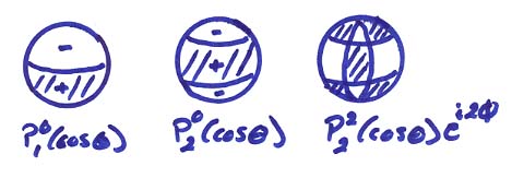
Examples of the vibrations of different spheroidal and toroidal modes are shown below.
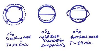
Ex)
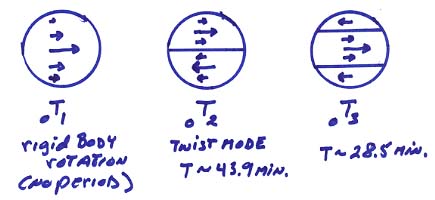
These are noted again as ![]() and
and ![]() where
where
n = the overtone number; the number of zero crossings in the radial direction in depth
l = the mode number; the number of nodes in latitude
m = the azimuthal order; the number of nodes in longitude
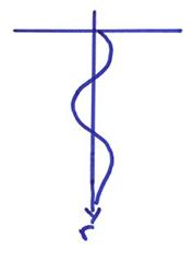
Ex) The amplitude
spectrum of the 1960 ![]() into two frequencies
at periods of 54.7 min. and 53.1 min.
This results in a waveform shown below due to interference between the
split modes.
into two frequencies
at periods of 54.7 min. and 53.1 min.
This results in a waveform shown below due to interference between the
split modes.
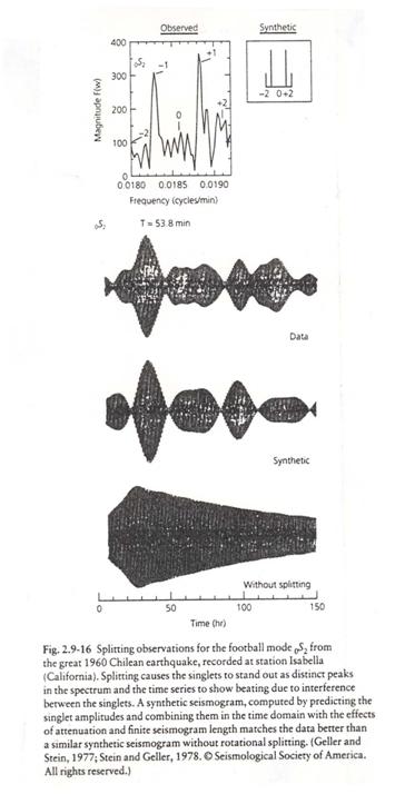
(from Stein and Wysession, 2003)
The width of the spectral peaks depend on the anelasticity of the Earth and also on whether or not the frequency resolution is fine enough to resolve additional “split modes” close to the mode corresponding to m = 0.
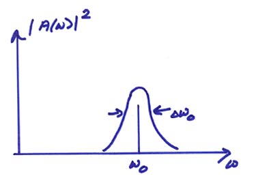
The width of the spectral peak can be written as ![]() where Q is the anelasticity factor.
Attenuation then decays the wave as
where Q is the anelasticity factor.
Attenuation then decays the wave as ![]() in time.
in time.
For the largest earthquakes, detectable long period ground motions can continue for several days. This is needed for the resolution of nodal peaks in spectrum. However, long period ground noise results in some limitations even for large magnitude events M > 8.
Technically, one can compute the entire seismogram by the synthesis of normal modes and this is now often done to compute seismograms which include the body waves. As we saw for the vibrating string, standing waves can be considered as a superposition of traveling waves. We might then guess that a normal mode of the Earth could be viewed as surface waves traveling in opposite directions over the Earth.
Ex)
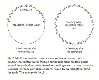
(from Stein and Wysession, 2003)
Below is a plot of the observed and calculated eigenfrequencies for the spheroidal and toroidal modes as a function of angular order l.
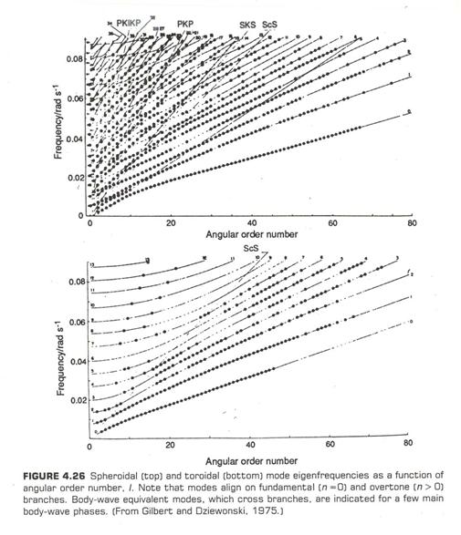
(from Lay and Wallace, 1995)
Below is a plot
of vertical component seismograms for the deep Columbian earthquake of
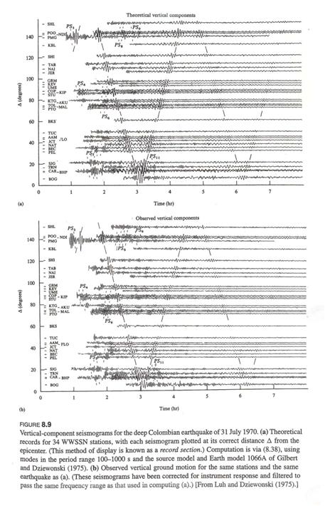
(from Aki and Richards, 2002)
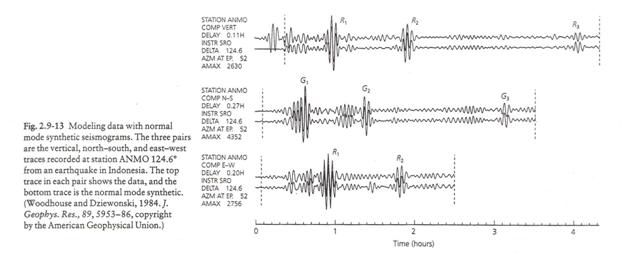
Below is a plot of normal mode seismograms for three source receiver pairs. The top trace for each is the observed and the bottom is the observed data. The Earth model is laterally varying obtained from a tomographic inversion. These types of data were used by Woodhouse and Dziewonski (1984) to perform one of the first tomographic inversions for upper mantle structure using normal modes.
(from Stein and Wysession, 2003)