EAS 557
Introduction to Seismology
Robert L. Nowack
Lecture 2
Linear Systems and Fourier Transforms
This lecture is adapted from some unpublished lecture notes by D.M. Boore and W. Thatcher.
References:
Bracewell, R. (1999) The Fourier Transform and its Applications, McGraw Hill.
Oppenheim, A.V., A.S. Willsky, et al. (1996) Signals and Systems, Prentice Hall.
Fourier Transforms
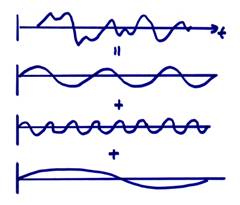
Fourier transforms are powerful tools and are used constantly by scientists and engineers. They connect two ways of looking at data in the frequency and in the time (or space) domains. A Fourier transform is simply a mathematical tool which enables any complicated function of, say, time to be written as a sum of sines and cosines of different “amplitudes” and “initial phases”.
The power in expressing a time domain signal in the frequency domain (via the coefficients or weights for the sines and cosines) is that certain numerical operations, such as differentiation and integration, are easy to carry out in the frequency domain.
We will define the transform pair
 “Fourier transform
pair”
“Fourier transform
pair” ![]()
(complex exponentials will simplify the algebra where ![]() = complex phasor
= complex phasor ![]() }.
}. ![]() ,
, ![]() radial frequency)
radial frequency)
Note that

Then we can write (1a) as

where  is the cosine
transform and
is the cosine
transform and  is the sine
transform. Real and imaginary parts of
is the sine
transform. Real and imaginary parts of ![]() are even and odd,
respectively, for a real signal g(t).
Thus,
are even and odd,
respectively, for a real signal g(t).
Thus, ![]() and
and ![]() .
.
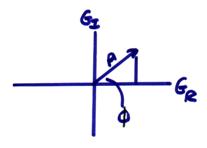
We can now
represent ![]() by its amplitude
and phase, as
by its amplitude
and phase, as
 for each
 ![]() .
.
Now lets use (1b), assuming g(t) is real, as


then,
 (1c)
(1c)
If g(t) is real, then ![]() is an even function
is an even function ![]() and
and ![]() is an odd
function. This will occur if
is an odd
function. This will occur if ![]() .
.
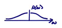
Thus, the amplitude (“spectra”) is symmetric (even) about ![]() , and the phase (“spectra”) is antisymmetric (odd) about
, and the phase (“spectra”) is antisymmetric (odd) about ![]()
for a real signal like a seismogram or a cardiogram. Thus, we will typically plot only ![]() for positive
frequencies (assuming real signals).
But, the negative frequencies must be included in any computations. From (1c), g(t) can always be
completely represented by a sum of weighted and shifted sines and cosines. This was not obvious to scientists of the 19th
century. But, information contained in
the waveform signal is often neatly summarized in the frequency domain.
for positive
frequencies (assuming real signals).
But, the negative frequencies must be included in any computations. From (1c), g(t) can always be
completely represented by a sum of weighted and shifted sines and cosines. This was not obvious to scientists of the 19th
century. But, information contained in
the waveform signal is often neatly summarized in the frequency domain.
Ex) Are there periodicities in the rotation of the Earth? Are there periodicities in the earthquake record?
Another important usage of Fourier transforms is that components of linear systems are easier to isolate in the frequency domain (i.e., your stereo system).
Linear Systems
Consider the following system for your stereo.
CD player ![]() preamp
preamp ![]() amp
amp ![]() filters
filters ![]() speakers
speakers ![]() audio output
audio output
This is similar to the earth, where for example
Earthquake source ![]() propagation in Earth’s
mantle
propagation in Earth’s
mantle ![]() propagation in Earth’s
crust
propagation in Earth’s
crust ![]()
recorded by seismometer ![]() visual output
visual output
A system can be written,
![]()
where g is the output signal and s is the input signal. It can also be written in input-output notation
![]()
We will restrict our discussion to linear and shift invariant systems.
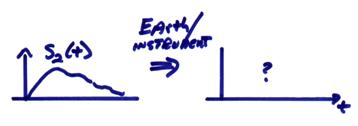
Consider an earthquake occurring in
the New Madrid, Missouri area of the
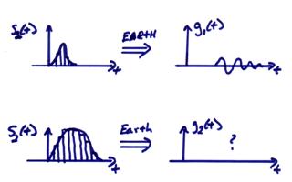
Is there enough information to predict the future ground motion g2(t) corresponding to a second, but larger, earthquake at the same location in New Madrid with a known rupture slip function on the fault, s2(t)?
Consider decomposing the input signal s into small rectangles
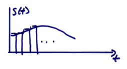
This can be written,
![]()
![]()
where ![]() is sometimes called a
“boxcar” function,
is sometimes called a
“boxcar” function,

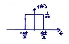
For a small ![]() , these boxcar functions would be skinny rectangles of unit
area.
, these boxcar functions would be skinny rectangles of unit
area.
Now, consider the output of our system

If the system T is “linear”, then for ![]() , then
, then
a) for a scalar ![]()
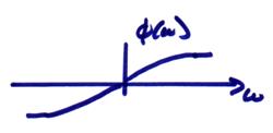
A simple way to think about this requirement for a linear system is that if you “double the input, you double the output”
b) for two input signals s1(t) and s2(t) with ![]() , then
, then ![]()
Note, the mathematical concept of linearity is subtle.
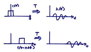
For a linear system then,
![]() (2)
(2)
where ![]() is the system function
T now acting on a series of time shifted “boxcars”. Thus, if we know the output of T for all the
skinny rectangles as inputs, we can find the output g(t) by adding up all the
outputs from the scaled skinny rectangles.
is the system function
T now acting on a series of time shifted “boxcars”. Thus, if we know the output of T for all the
skinny rectangles as inputs, we can find the output g(t) by adding up all the
outputs from the scaled skinny rectangles.
Now, we will make one final simplification.
Shift Invariance
A system T is shift invariant if for
![]()
then,
![]()
This assumes that the system (i.e., the Earth), hasn’t
changed in time ![]() . It is also sometimes
called time invariance. We can now write
(2) as
. It is also sometimes
called time invariance. We can now write
(2) as
![]() (3)
(3)
where ![]() is the shifted output
of a skinny rectangle of unit area as input.
In order to convert this to an integral, let
is the shifted output
of a skinny rectangle of unit area as input.
In order to convert this to an integral, let ![]() .
.
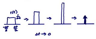
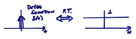
In the limit ![]() and is now called a “delta
function”.
and is now called a “delta
function”. ![]() is the delta function
response of the system T and is also called the “impulse response of system T”. Delta functions have 1) unit area, 2) no
width, and 3) infinite height.
Mathematicians in the past had difficulties with them, but these
functions are very useful.
is the delta function
response of the system T and is also called the “impulse response of system T”. Delta functions have 1) unit area, 2) no
width, and 3) infinite height.
Mathematicians in the past had difficulties with them, but these
functions are very useful.
We can then write (3) as an integral
 (4a)
(4a)
where g(t) is a sum of delta function outputs h(t) appropriately shifted in time and weighted by the source function amplitudes. This is called linear convolution and it is often abbreviated as
![]() (4b)
(4b)
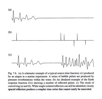
(from Shearer, 1999)
In the figure above, (a) represents the source s(t) from an airgun used in seismic exploration, and (b) represents an idealized Earth response function. (c) then shows the convolution of the source time function with the Earth’s response.
The important point is that if we know the output h(t) for an impulsive input,
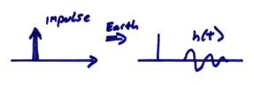
(i.e., the ground response at

All we know about the Earth is that an input impulse gives h(t) as output.
Now assume that our seismograph recording system is also linear/shift invariant, where
![]()
and

and if we substitute ![]() for g, then
for g, then
![]()
Thus, the power of the systems approach is that we can cascade the effect of subsystems by sequential convolutions with impulse responses of the different subsystems.
Now, the important connection with Fourier transforms is if

then
![]()
The convolution process is just multiplication in the frequency domain!
Proof
Let

where ![]() , then
, then
![]()

Let ![]() , where
, where ![]() is a “dummy variable” and
is a “dummy variable” and
![]() , then
, then
![]()

then
![]() .
.
Thus, convolution is just a multiplication of the respective
Fourier transforms frequency by frequency.
Finally, ![]() is obtained by the inverse
Fourier transform of
is obtained by the inverse
Fourier transform of ![]() back to the time
domain.
back to the time
domain.
Consider a cascaded system where we have a combined system
source ![]() Earth
Earth ![]() seismic instrument
seismic instrument
Then,
![]()
In the frequency domain this can be written as
![]()
Ex) Now, if we know the seismogram output y1(t) for a small earthquake with rupture time function s1(t)
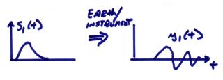
can we find the recorded output in ![]() , where
, where ![]() is assumed to be
given?
is assumed to be
given?
It turns out, yes, if the system is linear and shift invariant, but with qualifications. Then,
![]()
and,
![]()
If we form the ratio of the two Fourier transformed outputs,

then the Fourier components related to the Earth and the seismograph recording system cancel, assuming we don’t divide by zero in the process.
Then,
![]()
valid for ![]() , for all frequencies in the range of interest. We can thus find
, for all frequencies in the range of interest. We can thus find ![]() given
given ![]() , as well as
, as well as ![]() , without performing another experiment. This is the power of Fourier Transforms.
, without performing another experiment. This is the power of Fourier Transforms.
Since in the frequency domain, convolution can be written as
![]()
Deconvolution in the frequency domain is done by
spectral division for each frequency.
Thus, to find ![]() given
given ![]() and
and ![]() , then
, then
![]()
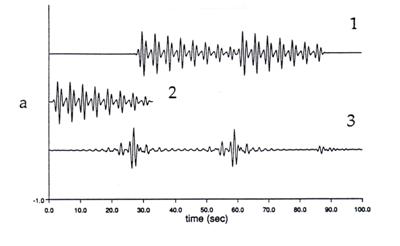
assuming ![]() . An example of this
is given in the figure below where 1) represents the output g(t),
2) represents the source s(t), and 3) represents an approximate
deconvolution of 1) by 2). Note that this
process can be unstable when
. An example of this
is given in the figure below where 1) represents the output g(t),
2) represents the source s(t), and 3) represents an approximate
deconvolution of 1) by 2). Note that this
process can be unstable when ![]() is near zero for some
frequencies.
is near zero for some
frequencies.
(from Erdogan, 1992)
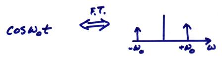
Finally, I give several examples of Fourier transform pairs
 a)
a)
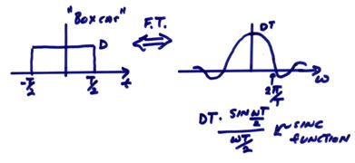
 b)
b)
 c)
c)
The “sinc function” is important for earthquake source problems and for seismic and optical diffraction problems.
Finally, I include several basic properties of Fourier transforms (see Bracewell, 1999 for more details). Below “FT” means taking the Fourier transform.
1) linearity ![]()
2) similarity ![]()
3) shift ![]()
4) Parseval’s theorem 
5) differentiation ![]()
6) convolution theorem ![]()