Purdue University

EAS 557

Introduction to Seismology

Robert L. Nowack

Lecture 3A

Seismometry 1

(This lecture adapted from unpublished lecture notes by D.M. Boore and W. Thatcher)

Recording ground motions from earthquakes or controlled sources is basic to almost all of seismology. Not surprisingly, seismology didn’t begin to develop as a science until the late 1800’s with the invention of the first reliable seismograph.

First, let’s look at the frequency range of interest.

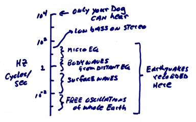
Besides this wide range of frequencies (five orders of magnitude for earthquakes), we also require a wide range of amplitudes.

The next figure shows the range of seismic ground displacements for different size earthquakes as a function of frequency and distance. For example, for teleseismic earthquakes, for magnitudes between 4 and 8, at a distance of (~ 10,000 km, where ~ 111.19 km), the range of ground motions at 1 Hz is from 10^-9 m (1 nanometer) to 5 x 10^-6 m (10^-6 m = 1 micron, where 2-3 microns is the size of a bacterium). At a lower frequency of .01 Hz, the range of ground motions can be from 1 micron to several cm’s for an earthquake of different magnitudes at teleseismic distances. For a small microearthquake of magnitude 2 at a distance of 30 km, the ground motions can be as small as 10^-9 meters or 10 Angstroms.

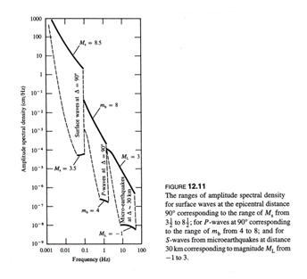
(from Aki and Richards, 1980)

No single instrument can record all these frequencies and amplitudes and even seismic recordings over a restricted frequency band-width are not completely faithful reproductions of the ground motion. Thus, any seismogram is a filtered version of the true motion, distorting it, but hopefully in a calculable way.

Although no longer in common usage, two types of mechanical seismometers illustrate the general principles without too much math.

1) The Mass and Spring System

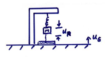
Here the ground moves through a displacement, u_G. The mass, M, is displaced by a relative amount u_r. Thus the total displacement of the mass, M, with respect to the fixed stars, say, is

Now, recall Newton’s 2^nd Law

.

where the inertial force is Ma. The restoring for the spring from Hooke’s Law is , where K is the spring constant. If the system has some damping, there will be a force due to damping of , where D is a damping constant. Then, from Newton’s 2^nd Law, the force balance will be

For and simplifying using , then

where and . This is a linear constant coefficient differential equation and is the forcing function. Thus, the output motion of the mass is related to the input ground acceleration through a differential equation.

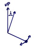
2) The Damped Pendulum System

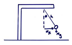
In this figure, . For small deflections, . The total motion of the pendulum bob is then

We can again use Newton’s 2^nd Law, F = Ma, where the inertial force of the mass is . The restoring force of gravity is , where g is the acceleration of gravity, 9.81 m/s². The damping force is . Finally, there is an additional reaction force at the support . The force balance can then be written as

or

.

The reaction force at the support can be written as

where is the radius of gyration. Then,

Let

Now, is called the “reduced length” of the pendulum. For the analysis here, we will just assume L ~ h. Then, we can write

This is very similar to the equation of motion of the mass and spring system.

Suppose we could amplify the pendulum deflection (using, for example, a light deflection from a mirror on the mass) by an amount . Then, let

then,

This has the identical form as the mass and spring seismometer system. It also includes a static magnification .

The Solution for Forced Response Systems

We will use Fourier transforms where a time derivative in the Fourier domain is equivalent to a multiplication by . Thus, we will write , where means in the time or frequency domains. Also, a second derivative, , corresponds to in the Fourier domain. We will investigate the generic forced response oscillator for both the mass and spring system and the small amplitude pendulum system as

(1)

I will first make several comments about the form of the solution to this differential equation.

For very rapid earth motion, the first term on the left side dominates and the mass motion is proportional to (by dropping the second two terms on the left side and integrating twice).

For very slow earth motion, the last term on the left side dominates and is proportional to the ground acceleration.

But the precise range depends on the value of the spring constant and thus of the undamped system ().

To obtain the frequency response input , write

and,

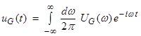
Then, substituting these into equation (1) and noting that each derivative introduces a (), we get

where the integral in frequency is brought out of the equation to the left. Since this must hold for all frequencies, the term in parentheses must be zero for each frequency. Then,

Converting this to real and imaginary parts

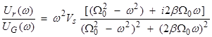
or in terms of amplitude and phase

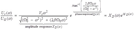
This gives the ratio of the oscillator response to the ground displacement at a given forcing frequency .

Of course, the actual ground motion is the sum or “Fourier integral” of the contributions over a range of frequencies. Each contribution is appropriately weighted by an amplitude factor and a phase factor. Finally, the mass response in the time domain can be obtained by inverse Fourier transforming to get . But, useful information can be obtained by looking just at the frequency response of the oscillator.

For and small damping, then and . Then, and the mass motion is proportional to ground acceleration as noted above (recall multiplication by in the frequency domain corresponds to taking a second derivative in the time domain). For and small damping, then and . For this case, recall that mass motion is proportional to the ground displacement (the frequency response is “flat”), but since is opposite in sign. Thus, when the ground goes up rapidly, the mass goes down. On a log-log plot, the amplitude response is

The phase response is

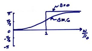
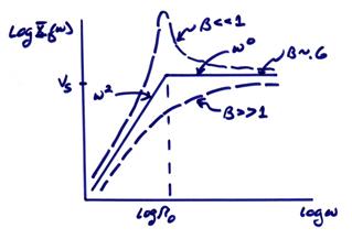
Note that is the resonant frequency of the oscillator. The free period is then . The mechanical oscillator is usually damped where ~ 0.6 is a commonly used damping since the amplitude response is simple, as shown above, where the response is

~ flat in displacement for

~ fall-off for

From the figure above, the other cases are

<< 1 – very little damping. This is called Richter’s “resonance catastrophy” since until about 1900 seismometers weren’t damped very much.

Can you guess what seismograms would look like?

>> 1 – overdamped. This is not used much since it reduces the overall response.

Now, let’s assume we want our seismometer to act as a “velocity meter”, then for ~ 0.6

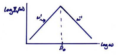
For this case, the velocity response of the system is

Note that using a log-log plot, this simply changes the slopes of the lines compared to the displacement response curve . Similarly, for an “accelerometer”

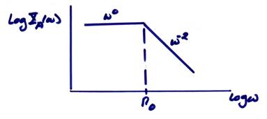
Note the simplicity of these response curves when we use log-log scales. Using relations,

then,

and

For these cases, log-log plots are very useful since powers of frequency plot as straight lines. Clearly the resonant frequency is the crucial parameter of the instrument response.

The free periods T₀ for the two different types of mechanical oscillators are:

Spring and mass

where M is the mass and K is the spring constant.

Damped pendulum

where L is the “modified length” of the pendulum and g is the acceleration of gravity. Again, for the analysis here, we assume L ~ h. As an example, if we wanted T₀ = 6 sec for a pendulum, which is a useful period for earthquakes, then L = 10 meters! Longer periods would be valuable to record too, but clearly this would get ridiculous fast.

Some early mass and spring seismometers used M ~ 20 tons to get longer free periods, but clearly K must increase too. Thus, there is a point of diminishing returns if we want the mass motion to be proportional to ground displacement.

For a pendulum, one answer is to reduce the gravitational restoring force by slightly inclining the pendulum on a rigid support, like a “garden gate”.

The restoring forces is then and effectively replaces in equation for T₀. (See also the Lacoste seismometer in Aki and Richards, 1980, Figure 10.3 for a vertical seismometer.)

Another alternative is just to record ground acceleration in which case T₀ can be small (and large). These types of mechanical instruments are called accelerometers.

Most modern seismograph systems employ mechanical components that are similar to the above mass and spring and pendulum systems. However, they are not used alone because their strictly mechanical nature severely limits 1) the free period, and 2) the static magnification. What we really want is a seismometer deflection that is proportional to some electrical signal that we can amplify and filter in ways we desire using well developed electronic techniques.