Purdue University

EAS 557

Introduction to Seismology

Robert L. Nowack

Lecture 4

Vector and Cartesian Tensor Analysis

References:

Schey, H.M. (1997) Div, Grad, Curl and All That, Norton.

Mase, G.E. (1970) Theory and Problems of Continuum Mechanics, Schaum Outlines, McGraw Hill.

Matthews, P.C. (1998) Vector Calculus, Springer-Verlag.

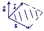
A vector in Euclidean space is a directed line segment with a given magnitude and direction.

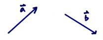
Certain physical quantities, such as force and velocity, which possess both magnitude and direction, may be represented in a three-dimensional space by directed line segments.

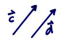
a couple of equal vectors

Below, I will give the vector notation to the left and the index notation for a Cartesian vector to the right.

; x_i i^th component of the vector

Vectors add according to the parallelogram rule

; (components add)

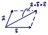
Put them head to tail to get the resulting vector addition.

Multiplication by a scalar , ;

Unit vectors with a unit length can be written , where

A vector is usually represented by a column. For example, here are the components of a vector in R³

There are several ways to multiply vectors.

1) The dot product between two vectors results in a scalar.

or in index notation

In index notation, repeated indices are dummy indices which imply

This is the so called Einstein sum convection. Note that .

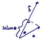
The geometric interpretation of the dot product is that it “projects” one of the vectors onto the other and multiples the resulting two lengths. Thus,

Ex) Let with

then,

Thus,

Note that for two vectors to be perpendicular to each other, then and .

2) The cross vector product between two vectors results in another vector, where

where is the measure area of parallelogram made from the two vectors and .

Use the right-hand rule to find orientation of .

This is an oriented vector depending on the order of the two vectors and follows a “right hand rule”. Thus, . A quick and dirty formula for the cross product can be obtained from the determinant as,

where

To express this in index notation, we must introduce the alternating symbol

then

where this has repeated indices on j and k and has an implied sum on them. Thus,

For example, for the c₁ component,

This is the same result as from the other formula. One of the reasons that a cross product has a complicated index notation form is that one is really trying to represent an area by a vector normal to it. This can be done in 3-D, but not in higher dimensions where the cross product cannot be represented as a vector, but rather the area itself must be used. This more general analysis is called the exterior calculus of differential forms.

3) The outer product results in a matrix type quantity of second order

In index notation, this is very simply written as

where i is the row index and j is the column index.

The volume of a parallel piped in 3-D is given by the scalar or

where a_i, b_j, and c_k are summed on i, j, and k. This results in

Thus, this determinant measures a volume.

A dyad is a second order tensor with two indices. A vector is a first order tensor and a scalar is a zero order tensor.

An identity matrix in R³ can be written as

This is often written as I or in index notation

and is called the Kronecker delta. A useful identity between the Kronecker delta and the alternating symbol is

A dyad can always be decomposed into its symmetric and an anti-symmetric part

where D^T is the transpose of D.

A linear transformation between two vectors can be represented by a dyad. Then,

In index notation, this is written

where there is an implied sum on j, or

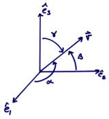
Coordinate Systems

In space, any vector can be represented as projections onto three non-zero, non-coplanar vectors. Let these be . These give a unique representation of any vector in 3-D. Then,

Most frequently, we will choose the rectangular Cartesian system () where , , and .

This forms an orthonormal set of basis vectors.

Now, the components of with respect to () are

In addition to rectangular Cartesian coordinates, we could (and will) use cylindrical systems (), spherical systems ().

For cylindrical coordinate systems

For spherical coordinate systems

Cylindrical coordinates Spherical coordinates

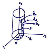
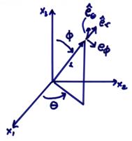
These systems provide unique representations, but, in general, do not have fixed directions in space and are functions of position.

Coordinate Transforms

The coordinate transformation from a vector from one coordinate system to another is given by the coordinate transformation equations

where are the coordinates of the vector in the x_i system and are the coordinates of the vector in the second system.

For small changes of the coordinates, use a Taylor series expansion as

(with an implied sum on j). This is an invertable transformation if is nonsingular.

Tensors will transform by

vector transformation

where are the components in coordinate system 2 and are the components in coordinate system 1. Second order tensors transform as

(implied sum on r and s).

In Cartesian coordinates, vectors transform from one rotated coordinate system to another as

(with implied sum on j) where are the direction cosines between and in the two coordinate systems. Thus,

where rotation matrices A = a_ij are orthonormal. Thus, and .

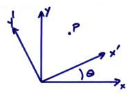
For example, for the point P, the coordinates in two rotated coordinate systems are related by

Second order Cartesian tensors transform like

(with implied sums on p and q). This in matrix notation is

General transforms are done using the Jacobian of the coordinate transformation equations and the introduction of a given metric. The components or “scale factors” (h₁,h₂,h₃) of the metric tensor come into the index description of the vector operations. (h₁,h₂,h₃) are the square root of the diagonals of the metric tensor. For example, for

Cartesian – h₁ = 1, h₂ = 1, h₃ = 1

spherical – h_r = 1, = r, =

cylindrical – h_r = 1, = r, h_z = 1

Vector and tensor fields assign a vector (or tensor) to every point in space (and time). Thus,

scalar field –

vector field –

tensor field –

Coordinate differentiation with respect to x_i is expressed by .

This is given a special symbol, the “del” or Nabla symbol. Thus,

Comma notation is sometimes used

Several important vector operations with del include,

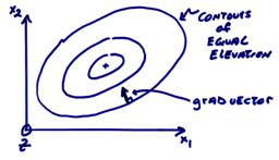
1) The del operator acting on a scalar field. This results in a vector field called the gradient or “grad”.

; (index notation)

For example, on a surface is the vector at that points in the direction of maximum ascent.

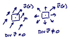
2) The del operator acting on a vector using a dot product results in a scalar field which is called the divergence or “div”.

In index notation, this can be written as or (sum on i). This measures the net flux into or out of the local region at a given point.

3) The del operator crossed with a vector in 3-D results in a vector field.

;

(index notation, sum on j and k) where is the alternating symbol. The curl measures the local vorticity or rotation (as in a bathtub drain) at a given point.

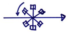
local paddle wheel

The curl points the direction of the rod for clockwise rotation.

4) The Laplacian is a second order operation

; (index notation, sum on i)

(sum on i).

5) Several identities of interest are

; (sum on j and k)

; (sum on i, j and k)

An essential integral identity is Gauss’ Theorem. This relates a volume integral to a boundary surface integral for a vector (tensor) field , where is the outward unit normal of the surface. Thus,

; (sum on i)

or for a second order tensor

Finally, we give the gradient, divergence, and curl in orthogonal curvilinear coordinates ()

where the h₁, h₂, h₃ are given for cartesion, cylindrical, and spherical coordinates above.