EAS 557
Introduction to Seismology
Robert L. Nowack
Lecture 6
Analysis of Stress
The concept of stress involves the action of forces on a body. Two types are considered:
1) Body forces – ![]() . Which are generally forces
per unit volume. For gravitational
forces, these depend on the mass distribution within the body. These are generally non-contact forces.
. Which are generally forces
per unit volume. For gravitational
forces, these depend on the mass distribution within the body. These are generally non-contact forces.
2) Surface forces – ![]() . These are forces per
unit area acting along surfaces of elemental volumes and are contact forces
with adjacent parts of the body. These
forces give rise to the concept of traction on external and internal
surfaces. The traction on an external
surface of the body is related to the applied force by
. These are forces per
unit area acting along surfaces of elemental volumes and are contact forces
with adjacent parts of the body. These
forces give rise to the concept of traction on external and internal
surfaces. The traction on an external
surface of the body is related to the applied force by
![]()
where ![]() is the average force
on the small surface
is the average force
on the small surface ![]() centered on the point
P.
centered on the point
P. ![]() is called the traction
vector.
is called the traction
vector.
Units of traction and stress are in force/area. In cgs, the units of stress are dyne/cm2. In SI, the units of stress are 1 Newton/m2 = 1 Pascal (1 Pascal = 10 dyne/cm2). Other units are
1 bar = 106 dyne/cm2 = 105 Pascals
1 bar = 1.0133 Atmospheres
1 kilobar = 15,000 lb/in2
We now want to investigate tractions on internal surfaces within a body. Consider a bar under tension
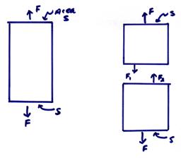
The external applied force, ![]() , results in tractions
, results in tractions ![]() on the ends.
on the ends.
Now, cut the bar and apply forces
on the two sides of the cut so that the shape of either section of bar remains
unchanged. Equilibrium requires that ![]() .
.
Now define
the tractions ![]() on the upper and lower
faces of the cut. From
on the upper and lower
faces of the cut. From ![]() . Thus,
. Thus, ![]() on the arbitrary
internal surface that we have constructed.
on the arbitrary
internal surface that we have constructed.
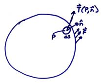
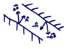
In 3-D,
consider a cut of area ![]() at a point P. Let
at a point P. Let ![]() be the force applied
to the side with normal
be the force applied
to the side with normal ![]()
Again, ![]() . On the other side of
the cut,
. On the other side of
the cut, ![]() .
.
From
![]()
Thus, as in the case for the bar, the tractions on either side of the cut are of the same magnitude, but opposite in sign.
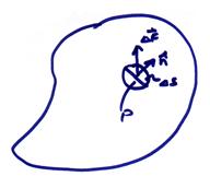
If we made cuts in other
directions, say with normals ![]() and
and ![]() , we would obtain different values for the internal traction
at P. Note that for a fluid, the
pressure is related to the traction by
, we would obtain different values for the internal traction
at P. Note that for a fluid, the
pressure is related to the traction by ![]() for any
for any ![]() . But in a solid, the
magnitude and direction of the traction depends on the orientation of the
surface element
. But in a solid, the
magnitude and direction of the traction depends on the orientation of the
surface element ![]() .
.
Ex) Consider the walls of a house.
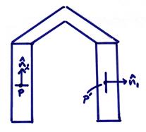
For an elemental area of the wall at point ![]() ,
, ![]() . But, at point P,
. But, at point P, ![]() will be non-zero and large.
will be non-zero and large.
It at first seems that there will be an infinite number of traction vectors at a given point depending on the orientation of the small surface. But, Cauchy proved, that in fact all the various tractions at P can be derived from a set of six numbers collectively grouped as the “stress tensor”.
Stress Tensor
The idea is instead of defining tractions on arbitrarily oriented planes at point P, we define tractions on the coordinate planes
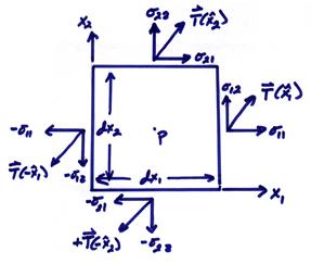
where
![]()
![]()
where ![]() and
and ![]() are unit vectors in
the x1 and x2 directions. The vectors are oriented in the conventional
positive directions. Thus,
are unit vectors in
the x1 and x2 directions. The vectors are oriented in the conventional
positive directions. Thus, ![]() would be positive if
they stretch the material. Also, on the
opposite faces
would be positive if
they stretch the material. Also, on the
opposite faces
![]()
![]()
In 3D, we will write
in which ![]() is the stress tensor
at the point P, where
is the stress tensor
at the point P, where
![]() are tensional or compressive
stresses
are tensional or compressive
stresses
![]() are shear stresses
are shear stresses
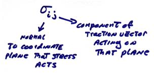
In index notation, the stress tensor is ![]() , where i is normal
to coordinate plane in which the traction acts and j indicates the component of the traction vector.
, where i is normal
to coordinate plane in which the traction acts and j indicates the component of the traction vector.
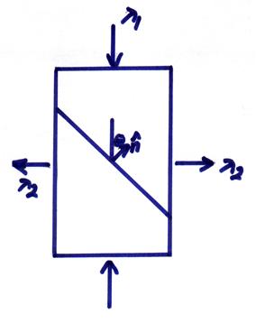
Cauchy showed that the stresses on any plane through an internal point P can be written as a linear combination of the elements of the stress tensor. This is a fundamental theorem of solid mechanics. Consider the triangle in 2D (tetrahedron in 3-D)
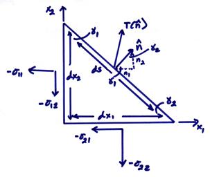
The traction on surface with normal ![]() is
is
![]()
.
Now we must find the condition of equilibrium of the triangle. Balancing forces in the x1 and x2 directions gives
In the x1 direction: ![]()
In the x2 direction: ![]()
or
![]()
![]()
From geometry
![]()
![]()
We then find
![]()
![]()
In index notation for 3-D, then
 (with implied sum
on j)
(with implied sum
on j)
Thus, the knowledge of the stress tensor ![]() specifies completely
the state of stress around the point P.
specifies completely
the state of stress around the point P.
In order to prevent the body from spinning, we also require that the net torque be zero. Evaluating the torque for a reference point at the center of the square, we get
![]()
where ![]() is a force and
is a force and ![]() is a moment arm. Then,
is a moment arm. Then, ![]() .
.
In the general 3-D case, ![]() . Because of this
relation, the stress tensor is symmetrical, where
. Because of this
relation, the stress tensor is symmetrical, where
with ![]() ,
, ![]() , and
, and ![]() . Thus, only six
numbers are needed to completely describe the state of stress of an internal
point P in a body.
. Thus, only six
numbers are needed to completely describe the state of stress of an internal
point P in a body.
It is important to separate between
the isotropic and deviatoric part of the stress tensor ![]() . We define
. We define
![]()
where ![]() is independent of the coordinate
system and P is the pressure. The minus
sign is used to require P to be positive when it is compressive. The stress elements themselves are positive
in tension. We rewrite
is independent of the coordinate
system and P is the pressure. The minus
sign is used to require P to be positive when it is compressive. The stress elements themselves are positive
in tension. We rewrite ![]() as
as
![]()
or in index notation
![]()
where ![]() is the deviatoric part
of the stress tensor.
is the deviatoric part
of the stress tensor.
For hydrostatic
stress, ![]() . For a hydrostatic
increase of stress with depth due to a uniform overburden, then
. For a hydrostatic
increase of stress with depth due to a uniform overburden, then
![]()
where ![]() is the density of the
overburden, z is thickness, and g is the acceleration of gravity. As an example, the hydrostatic pressure at a
depth of 10 km underneath a thickness of rock with an average density of 3000
kilograms/m3 is
is the density of the
overburden, z is thickness, and g is the acceleration of gravity. As an example, the hydrostatic pressure at a
depth of 10 km underneath a thickness of rock with an average density of 3000
kilograms/m3 is
P = (3000 kilograms/m3) (10 x 103 m) (9.8 m/s2)
= 2.94 x 10⁸ Pascals ~ 294 MPa
= 2.94 kbars
At an average thickness of the crust of 30 km, the hydrostatic pressure would be on the order of 1 GPa or 10 kbars.
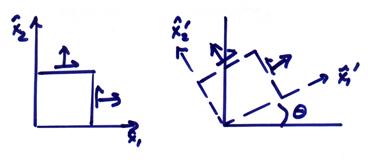
Transformations of
the Stress Tensor in Rotated Coordinate Systems
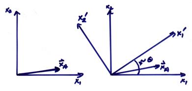
The
components of a vector in a rotated coordinate system can be related to the
components in the original system by a coordinate rotation matrix ![]() . For example, the
components of the vector
. For example, the
components of the vector ![]() above, in two
coordinate systems, can be written
above, in two
coordinate systems, can be written
![]()
where the components of ![]() are the direction
cosines between the old and new coordinate axes. The rotation matrix is,
are the direction
cosines between the old and new coordinate axes. The rotation matrix is,
![]()
As an example, if ![]() , then
, then
![]()
Let ![]() , then
, then ![]() in the new coordinate
system.
in the new coordinate
system.
Note for rotation matrices, ![]() since these are
orthogonal matrices. Now assume a
general relationship between two vectors
since these are
orthogonal matrices. Now assume a
general relationship between two vectors ![]() and
and ![]()
![]()
In a rotated coordinate system
![]()
Then, the general relationship between ![]() and
and ![]() can be written
can be written
![]()
or
![]()
Thus, ![]() in the new coordinate
system where
in the new coordinate
system where ![]() with
with ![]() . This general
relationship has the same form in any rotated coordinate system with the coefficients
depending on the orientation of the coordinate system.
. This general
relationship has the same form in any rotated coordinate system with the coefficients
depending on the orientation of the coordinate system.
Now,
consider the traction vector on an internal plane with normal ![]()
![]()
Since ![]() , this can also be written
, this can also be written
![]() or
or ![]()
In a rotated coordinate system, the traction vector is
![]() with
with ![]()
Now, we
choose ![]() so that
so that ![]() is a diagonal
matrix. In this special coordinate
system, all the shear stresses are zero and the normal stresses are called the principle stresses acting with respect
to the three rotated coordinate axes.
Let
is a diagonal
matrix. In this special coordinate
system, all the shear stresses are zero and the normal stresses are called the principle stresses acting with respect
to the three rotated coordinate axes.
Let
where ![]() are the rotated axes
with respect to the unrotated axes.
Then,
are the rotated axes
with respect to the unrotated axes.
Then, ![]() can be written as
can be written as
or for each ![]() , then
, then
![]()
forms an eigenvalue problem.
To find the eigenvalues ![]() , the determinant of
, the determinant of ![]() must be zero. Thus,
must be zero. Thus,
to solve for ![]() . Next solve for the
eigenvectors
. Next solve for the
eigenvectors ![]() and make sure to
adjust
and make sure to
adjust ![]() to unit length. Standard computer software, such as Matlab,
can be used to find the principle stresses
to unit length. Standard computer software, such as Matlab,
can be used to find the principle stresses ![]() and the principle
stress directions
and the principle
stress directions ![]() (i = 1,3).
(i = 1,3).
These can
be ordered such that ![]() . Since these are
positive for tensional stresses,
. Since these are
positive for tensional stresses, ![]() provides the maximum
compressive stress. There are no shear
or tangential stresses act on these new coordinate faces, only normal stresses.
provides the maximum
compressive stress. There are no shear
or tangential stresses act on these new coordinate faces, only normal stresses.
In the 2-D case, it is useful to derive these relations in detail
Let ![]() where
where  ,
, ![]() , and
, and ![]() . Then,
. Then,
This can be multiplied out and written in terms of
components of ![]() as
as
![]()
![]()
![]()
If we let ![]() , then we can find the rotation angle
, then we can find the rotation angle ![]() to be
to be
![]()
Since
![]()
If ![]()
![]() , then,
, then, ![]() will be the maximum
and minimum normal stress. Thus,
will be the maximum
and minimum normal stress. Thus,

These would then be the eigenvalues in the above eigenvector
analysis in 2D. From ![]() , we find that
, we find that

on planes with normal 45o from the maximum compressive stress direction.
This gives rise to the simplest theory of faulting where shear failure occurs on planes of maximum shear stress with normals at 45o from the axis of maximum compressional stress.
If rocks possess a cohesive strength and internal friction,
the angle ![]() will generally be
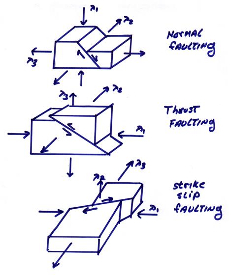
different from 45o. In 3D,
different regimes of faulting can be inferred depending on the orientations of
the principle stress directions
will generally be
different from 45o. In 3D,
different regimes of faulting can be inferred depending on the orientations of
the principle stress directions
For example, normal faulting, thrust faulting, and strike-slip faulting result when the principle stress directions are oriented as below.
As an example of the calculation of the principle stresses in 2D, let
![]()
then,
![]()
![]()
This gives for the principle stresses,
![]()
![]()
Thus,
Then
![]() and
and ![]()
These must then be normalized to unit length to get ![]() and
and ![]() . Using the 2-D
formulas
. Using the 2-D
formulas

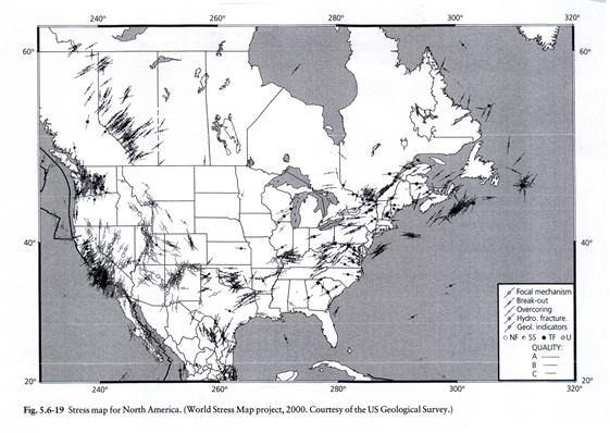
Stress maps showing the orientation of maximum horizontal shear stress have been developed based on orientations of earthquake faulting and in situ stress measurements. One technique for finding this is from breakout zones in boreholes which align with the principle stress directions and are often consistent over regional distances.
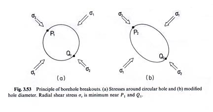
(from Meisner, 1986)
A second in situ approach uses the method of hydraulic fracturing in boreholes in which the induced fractures often align with the regional stress direction.
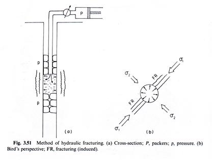
(from Meisner, 1986)
An example map of maximum horizontal compressive stress is shown below.