EAS 657
Geophysical Inverse Theory
Robert L. Nowack
Lecture 1
INTRODUCTION
Understanding the physical nature of the earth requires the development of physical models. A first step is to develop mathematical representations of earth properties. Examples of these include:
The temperature distribution
The seismic velocity structure
The density structure
There are also physical observables connected to each of these properties. Examples of these include:
heat flow
the seismic wavefield
the gravity field
Given a "model" of one of these properties, it is possible to calculate the corresponding values of the observable using a "physical law". Examples of these include:
Heat conduction equation
Seismic wave equation
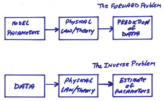
The "forward problem" connects the properties of the medium with the observables.
How do we represent the physical parameters of the model? The possibilities include:
1) Values of earth properties at all points in the medium (this is unwieldy)
2) Functional representations, such as spherical harmonics (coefficients)
3) Values at discrete points (which can then be interpolated)
4) Values within discrete layers or "chunks"
Most geophysical model representations fall into the last three. Generally the coefficient/discrete chunk values are called the model parameters.
In geophysical inverse theory, the model parameters need to be determined given a set of observables (data) and a physical law or theory. In addition, one needs to estimate the model parameter errors and the model resolution.
The forward and inverse problems are shown below.
Geophysical inverse theory can also be looked at in terms of a boundary value problem and an inverse boundary value problem. This again assumes a physical law/theory.
|
|
B.V.P. |
Inverse B.V.P. |
|
Given: |
1) properties of the medium |
2) sources |
|
|
2) sources |
3) measurements on the boundary |
|
|
3) measurements on the boundary |
(for each source) |
|
Find: |
Field values inside boundary |
Properties of medium field values inside the |
|
|
(solve the forward problem) |
boundary (inverse problem) |
Despite the apparent difficulty in solving the inverse problem, in practice one of the hardest steps is formulating and solving the forward problem. Once the sensitivity of how the medium parameters influence the observations is found, a procedure can be developed to find the medium properties that can explain the observations. But, finding a solution is only the beginning of the inverse problem. It is even more important to understand the range of possible solutions. Thus, inverse theory is also the study of how well various models explain the data.
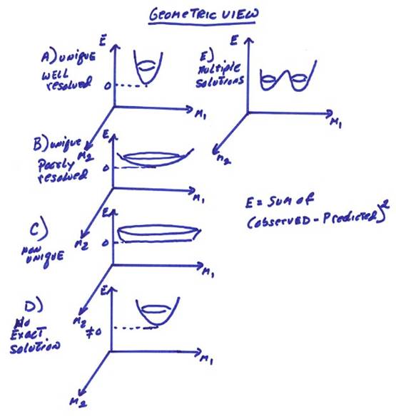
There are two viewpoints. First there is the geometric approach (in a suitable Hilbert space). The figure below gives several examples of uniqueness, resolvability, and multiple solutions where M1 and M2 are model parameters and E is a measure of the fit between the observed and predicted data.
The second viewpoint uses probabilistic concepts. In the figure below, the model and the data are plotted as a probability density distribution centered on the observed data and prior model. The forward problem is given by g(m) = d and a model is desired that maximizes the probability and also solves the forward problem.
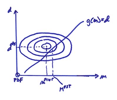
The two viewpoints (geometric and probabilistic) are not exclusive since the length measure of the error E can incorporate probabilities. But, a solution of an inverse problem without an understanding of the non-uniqueness aspects is usually worse than no solution at all since it may lead to an unwise decision.
As an example, Eratosthenes (~250 B.C.) attempted to measure the radius and circumference of the earth. He used the following observations.
At
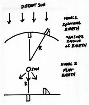
Thus, by assuming a spherical
model for the Earth and using similar triangles as in Model 1 above, he derived
that the ratio of the distance between the two cities to the radius of the
earth was also 1/8. From this, he found the
Earth’s radius R and a circumference of 24,700 miles. This had a precision which was not exceeded until
However, this analysis is model dependent. If the model is assumed to be a flat Earth and light rays are diverging from the Sun, as in Model 2 above, the inferred R is the distance to the Sun. Thus the data can be exactly fit with two completely different models. It was part of the brilliance of Eratosthenes to pick the correct model.