EAS 657
Geophysical Inverse Theory
Robert L. Nowack
Lecture 10
In the Bayesian method assuming Gaussian statistics, we want to find x such that the pdf of the model given the data is maximized. For a linear forward problem,
![]()
This pdf is maximized if the combined exponent term is minimized. Thus,
![]()
This assumes that the data and model residuals y – Ax and (x-x0) follow Gaussian distributions. In the maximum likelihood method, only the first term is minimized and thus Gaussian statistics is associated with weighted least squares. In Bayesian statistics, the two terms are simultaneously minimized.
We will first investigate the statistics involved with the maximum likelihood method and later with Bayesian inversion.
Ex) Find the errors in the model from errors in the data where
![]()
The covariance matrix for errors in the model from the data errors is

where < > denotes the average
and ![]() is an outer
product. If the yi’s are independent and
identically distributed (i.i.d.), then
is an outer
product. If the yi’s are independent and
identically distributed (i.i.d.), then
![]()
and
![]()
where ![]() is the unit covariance
operator Cu. For Case 3a) described
earlier where N(A) = {0}, then
is the unit covariance
operator Cu. For Case 3a) described
earlier where N(A) = {0}, then
![]()
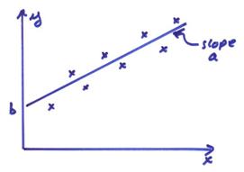
Ex) Ax
= y resulting from fitting a
line to points as y = a x + b or

where b is the intercept and a is the slope
The errors in (b,a) resulting from the data errors are given by
![]() where
the model parameters are
where
the model parameters are ![]()
and


and
![]() .
.
Thus, the magnitude of the errors in a and b are dependent on <x2>. If the range of x is small, then <x2>
~ <x><x>, resulting in a large magnification of the errors. There is also a cross term ![]() and the correlation
coefficient is
and the correlation
coefficient is
![]()
This gives
![]()
If <x> = 0,
then a and b are uncorrelated. This results if the data is centered about x = 0.
If <x> ![]() 0, and if <x2> is small, then there
will be a strong negative correlation between slope and intercept (b,a). Thus, it is important to center the data
about x = 0 when performing a line
fit.
0, and if <x2> is small, then there
will be a strong negative correlation between slope and intercept (b,a). Thus, it is important to center the data
about x = 0 when performing a line
fit.
Ex) For the averaging of M numbers yi with ![]() , then
, then

In the maximum likelihood method, we want to find <y> that maximizes this pdf. We can also minimize the exponent
![]()
and this minimizes the sum of the
squares. For two measurements, y1 and y2, this is
![]()
or
![]()
which is the average of the two
values. The values y1 and y2
are thus equally weighted. Suppose the
error in y1 is ![]() 1 cm and the error is y2
is
1 cm and the error is y2
is ![]() .1 cm. We can use the reciprocal
of data covariance matrix as the weights where
.1 cm. We can use the reciprocal
of data covariance matrix as the weights where
![]()
Then,
![]()
and
![]()
Now, we have weighted the measurement y2 by 100 times over y1 in the average.
In Bayesian inversion using Gaussian statistics, we would like to simultaneously minimize both

Minimizing the second term minimizes the weighted model norm.
Ex) Assume the model parameters are

For example, chose the prior values and uncertainties as
![]()
![]()
![]()
Note that these do not have the same physical units or
dimensions. We will use ![]() to equalize the
weights. Let
to equalize the
weights. Let

The minimization of the model norm would give
Min: 
Thus, we would minimize
![]()
Ex) Assume a layered model where some layers are thin and some are thick. For a minimum model norm, then
Minimize: ![]()
or by discrete analogy,
Minimize: ![]()
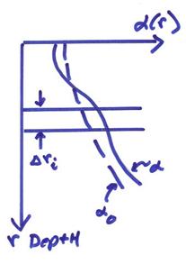
Note that here ![]() is an implicit weighting
function. The larger
is an implicit weighting
function. The larger ![]() is the more weight. A similar implicit weighting by block size or
volume occurs in higher dimensions.
is the more weight. A similar implicit weighting by block size or
volume occurs in higher dimensions.
We want to generalize the results when
![]()
For the Bayesian or stochastic inversion assuming Gaussian statistics, we want to find the minimum of
![]()
Thus, given the observed data y and the data covariance matrix Cd, we also need the prior information,

We will first investigate the problem graphically. Since the prior model distribution is assumed to be independent of the actual data values, then the joint pdf of y and x is
![]()
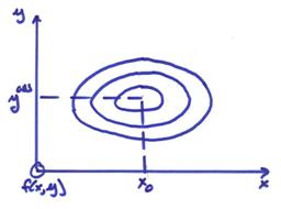
We have yet to introduce our knowledge of the forward problem (the relation between data and model). A linear relation, Ax – y = 0 defines a hyperplane in (x,y) space. In general, we may have a nonlinear relation between x and y or g(x,y) = 0 or y = g(x).
We now want to find (xest,ypre) such that
1) g(xest,ypre) = 0
2) maximize the joint pdf f(x,y)
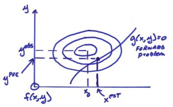
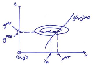
If g(x,y) = 0 is satisfied only for one point such that f(x,y) is maximized, then this is a unique solution. However, we can have several different situations that could occur. These are two end members cases that can occur.
A) The prior model
parameters are much more certain than the observed data yobs, then
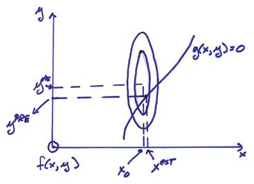
xest is near the prior model x0.
B) The prior model
parameters are much less certain than the observed data yobs, then xest
can be farther away from x0.
Using Bayes Theorem, we can obtain the posterior distribution from

For Gaussian statistics for the data and prior model and a linear forward problem y = Ax, then
![]()
The maximum of the posterior distribution for x can be found by maximizing this distribution or minimizing the exponent. Thus
![]()
Assume, for
simplicity, that the parameters and data are real valued. Let ![]() and
and ![]() , then using index notation
, then using index notation
![]()
where repeated indices in individual terms imply summation and both C and D are symmetric where

Then,
![]()
![]()
In vector notation this can be written
![]()
and
![]()
This results in
![]() (1a)
(1a)
This is called the stochastic inverse based on Bayesian analysis. This can also be written as
![]() (1b)
(1b)
Ex) Let ![]() . If the data is very
inexact, then
. If the data is very
inexact, then ![]() . From Eqn. (1a)
. From Eqn. (1a)
![]()
For this case, the data provides no constraints and the best solution is the prior model.
Ex) Let ![]() . If the prior model
is very inexact, then
. If the prior model
is very inexact, then ![]() , and
, and
![]()
then,
![]()
This is weighted least squares solution. If ![]() , then
, then
![]()
This is the standard least squares solution.
Ex) If ![]() and
and ![]() , then
, then

If  , and for
 ![]() , this results in the damped least squares solution,
, this results in the damped least squares solution,
![]()
Thus, the stochastic inverse “damps” out those eigenvectors that would give rise to perturbations in x larger than the prior model variance. The eigenvectors associated with very small eigenvalues are reasonably taken care of by the use of damping without resorting to the singular value decomposition.
For the stochastic inverse, the
resolution matrix ![]() is a distorted version
of [VpVp*] and also I-R is a
distorted version of {V0V0*}. But, if the damping is not too severe, R is
still a useful approximation to the resolution matrix.
is a distorted version
of [VpVp*] and also I-R is a
distorted version of {V0V0*}. But, if the damping is not too severe, R is
still a useful approximation to the resolution matrix.
As ![]() in the damped least
squares is changed from 0 to
in the damped least
squares is changed from 0 to ![]() , then the graph below results
, then the graph below results
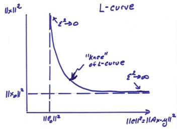
where
![]()
This is called
the “L-curve” by Hansen (1998) (“Rank-Deficient and Discrete Ill-Posed
Problems”,
The resolution and covariance matrices can be written as
![]()
![]()
where the term ![]() results from the
amplification of the data errors back to the model by
results from the
amplification of the data errors back to the model by ![]() and
and ![]() is projection of the
prior model covariance and errors onto the null space of A.
is projection of the
prior model covariance and errors onto the null space of A.
For the stochastic inverse,
![]()
and
![]()
The resolution matrix can then be interpreted as a filter resulting in the estimated model parameters x.
![]()
Now,
![]()
![]()
Then,
![]()
Note these
forms for ![]() are a formal composite
of both data and remaining prior model errors in the stochastic inverse
formulation. Also, the form
are a formal composite
of both data and remaining prior model errors in the stochastic inverse
formulation. Also, the form ![]() is not valid in the
least squares limit where R = I and the other form should be used
operationally. For the case where
is not valid in the
least squares limit where R = I and the other form should be used
operationally. For the case where ![]() , then
, then ![]() approaches the
weighted least squares limit for the model covariance.
approaches the
weighted least squares limit for the model covariance.
Data statistics can often be determined experimentally. But, model probabilities are purely subjective and one must beware of personal bias. Another hidden pitfall is if the forward modeling matrix A is incorrect. Difficulties will arise if the underlying model structure that was used to determine A is unrealistic.
Ex) A common structural model is a layered Earth and many false conclusions in geophysics have resulted from this assumption.
There are
two alternative forms for the stochastic inverse. First, the following identity is true for
positive definite covariance matrices ![]() and
and ![]() .
.
![]()
This can be shown by manipulating to get the identity
![]()
Starting with Eqn. (1b) given earlier, we can get the alternative form
![]() (1c)
(1c)
This form results in the inversion of an MxM matrix instead of an NxN matrix and is commonly used when there are less data than model parameters since the matrix to be inverted is smaller. The two forms in equations (1b) and (1c) can be used depending on whether the model or data spaces are larger.
The stochastic inverse is the most sensible approach to an inverse problem provided the covariances (or probability distributions) are known or can be estimated. It can be viewed as a damped least squares solution and one can show that a little damping is always useful.
For these discussions, it is useful to renormalize our data and parameters so that they have unit variance, a very useful numerical procedure!
Consider the data covariance matrix
![]()
Define
![]()
Also consider the prior model covariance matrix
![]()
Define
![]()
Now let
![]()
This results in the weighted forward problem
![]() .
.
The stochastic solution for the linear case given earlier, can be written either as
Form A) ![]() (Eqn. 1b)
(Eqn. 1b)
or
Form B) ![]() (Eqn. 1c)
(Eqn. 1c)
The reweighted problem can be written in terms of
![]()
Then,
Form A1) ![]()
Form B2) ![]()
and ![]() . The solution to the
original problem is then found from
. The solution to the
original problem is then found from
![]()
![]()
Nonlinear Problems
For nonlinear problems g(x,y) = 0 and y = g(x), complicated multi-minimum error surfaces can often occur as shown in the figure below.
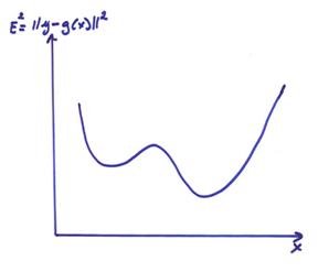
Most direct methods for solving nonlinear problems require
the sampling of the error surface by many calculations of the forward problem
and evaluating the error ![]() to find the
minimum. Different methods include:
to find the
minimum. Different methods include:
1) The grid search method. In this approach, the model space is
uniformly sampled in order to find the smallest ![]() . Unfortunately, this
method is very slow for model spaces with many parameters.
. Unfortunately, this
method is very slow for model spaces with many parameters.
2) The ![]() .
.
3) The Simulated Annealing Method. In this approach, an analogy to thermodynamics is used to restrict the area searched in the model space depending on a decreasing “temperature” parameter.
4) Genetic Algorithms. In these approaches, an analogy to genetics in biology is used to select regions of the model space to sample.
These approaches are all ongoing areas of research and I refer to Sen and Stoffa (1995) “Global Optimization Methods in Geophysical Inversion” Elsevier, for more details.
A gradient
style approach can also be used similar to
For the nonlinear case, use a

To first order, this can be truncated to the first two terms. Let  evaluated at xk
be the linear sensitivity matrix or Fréchet
derivative for the nonlinear operator g(x). Using a Bayesian approach, an iterative
algorithm is then obtained as,
evaluated at xk
be the linear sensitivity matrix or Fréchet
derivative for the nonlinear operator g(x). Using a Bayesian approach, an iterative
algorithm is then obtained as,
![]()
This can also be written in normalized forms (see, Tarantola, 1987). The second term in the brackets is zero for the first iteration, but is non-zero for higher iterations. This term has the function of keeping the solution referenced to the original prior x0 and it’s uncertainty.