EAS 657
Geophysical Inverse Theory
Robert L. Nowack
Lecture 11
3-D Teleseismic Inversion of Travel Time Data
The use of seismic travel-time data has been the classical way to study Earth structure since the advent of seismology.
Ex) Jeffrey and Bullen, as well as Gutenberg, developed radial earth models and used these to predict seismic arrival times starting in the 1930’s. More recent radial earth models include PREM and IASP91.
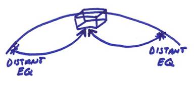
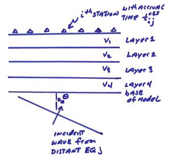
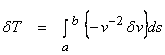
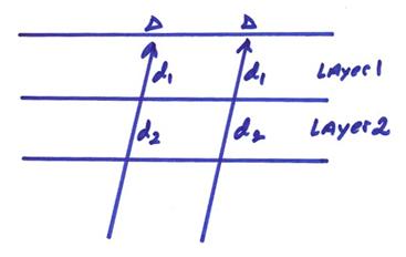
Aki (1977) and others developed tomographic methods to estimate variable 3-D earth models beneath large aperture seismic arrays including NORSAR and LASA using teleseismic travel-times. The method is now called the ACH method after Aki, Christoffersson and Husebye. The idea is to use a standard radial earth model for the mantle structure and choose teleseismic earthquake sources over a wide azimuth range to average out deeper upper mantle variations. This is then used as a starting model to determine the local crust and mantle laterally homogeneous structure beneath the array. The starting layered earth model beneath the seismic array is shown below with an incident teleseismic plane wave.
We will calculate travel times through the initial earth
structure from each earthquake to each station ![]() and compute the observed
minus calculated residuals,
and compute the observed
minus calculated residuals, ![]() .
.
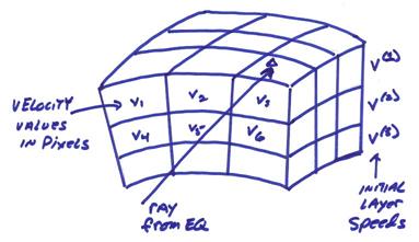
The idea is to break up the local crust and mantle structure beneath the receivers into a number of blocks and determine the velocity perturbations that will result in minimum residuals between the observed and calculated arrival times.
Note the following points:
1) Perturbing all velocities in one layer changes all calculated arrival times for a given earthquake by a constant amount.
2) This is the same as changing a distant time parameter from the source crust, lower mantle, or the earthquake origin time.
3) We can only minimize relative residuals about some given trial model and this has an inherent non-uniqueness. This reveals itself for this problem as one zero eigenvalue per layer.
For the jth event and the ith station,
![]() higher order terms
higher order terms
where ![]() is earthquake origin
time perturbation (or perhaps an event mislocation or source crust, and mantle
heterogeneity), Vk is the derived solution, and V(l) is
layer starting velocity.
is earthquake origin
time perturbation (or perhaps an event mislocation or source crust, and mantle
heterogeneity), Vk is the derived solution, and V(l) is
layer starting velocity.
How do we calculate ![]() ?
?
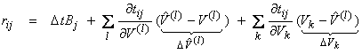
The depth and distance of the earthquake source determines the angle of incidence of a plane (P-wave) incident at the base of the model.
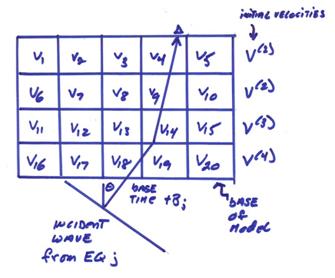
Then, follow the ray through the model using Snell’s Law. For the ray in the above figure,
![]()
where dK is the ray distance traveled in each block and tB is the arrival time at the base of the model. Assuming a starting radial model for the velocities,

the partial derivatives are then,

where V(l) is the starting layer velocity. Note that this approach is the correct one since perturbations of the travel time due to changes of the ray path are second order effects. Thus for
then,
where the integral is along the unperturbed ray path. Now the residuals can be written as
![]()
where ![]() is earthquake source
and distant path residual,
is earthquake source
and distant path residual, ![]() is a sum over the sampled blocks, and nij is a noise vector.
Also,
is a sum over the sampled blocks, and nij is a noise vector.
Also,
![]()
and

where V(l) is the layer velocity related to the block index k.
In order to separate the problem of
uniform perturbation terms ![]() , use the following trick
, use the following trick
The term  is zero if
 ![]() . Thus, we have added and subtracted
. Thus, we have added and subtracted ![]() , so
, so ![]() represents the perturbation
of the average layer velocity.
represents the perturbation
of the average layer velocity. ![]() represents the differences
between the block velocities and the unknown average layer velocity. Now compute <rj>, the mean residual for event j over all stations
represents the differences
between the block velocities and the unknown average layer velocity. Now compute <rj>, the mean residual for event j over all stations
where N is the number of stations. Now ![]() and
and ![]() are the same for all
stations for one event since the di
are the same.
are the same for all
stations for one event since the di
are the same.
Then,
where <ajk> is equal to
![]()
which is the “average partial derivative” for that block. Then,
where ![]() .
.
Thus, in order to set up the problem for the inversion of the block velocities from some unknown layer velocity,
1) Collect the observed
travel times for each event j at
stations i.
2) Compute the calculated
times, and residuals ![]() .
.
3) Compute ![]() the average residual over
all stations from one event, and
the average residual over
all stations from one event, and ![]() .
.
4) compute ![]() and
and ![]() and
and 
We have then gotten rid of both the statics term tBj and the uniform layer perturbations from the problem and are now only inverting for the perturbations from some unknown uniform layer velocity. Construct the matrix equation
![]()
where R is the vector of relative residuals, A
contains the “relative” partial derivatives and ![]() are the velocity
perturbations from some unknown layer velocity.
Thus,
are the velocity
perturbations from some unknown layer velocity.
Thus,
![]()
although we will typically use a stochastic inverse to compute this.
There are additional problems when using this approach, including
1) Is the problem really linear? Changing the V(l) will, in fact, change and bend the ray paths. We appeal to Fermat’s principle for small perturbations to utilize the original unperturbed ray paths.
2) Small singular values are always present and damping is usually needed. Some rays may have identical ray paths.
3) There may be structures directly below the model which could still possibly affect the relative residuals. The depth of the model to be inverted is important.