EAS 657
Geophysical Inverse Theory
Robert L. Nowack
Lecture 12
From an earlier lecture, we showed that the stochastic inverse solution minimizes
![]()
where x are
the model parameters, x0
are the prior model parameters, ![]() and
and ![]() are the data and prior
model covariances, and g(x) is the predicted solution to the
forward problem g(x), where this is, in general,
nonlinear.
are the data and prior
model covariances, and g(x) is the predicted solution to the
forward problem g(x), where this is, in general,
nonlinear.
A linearization procedure involves
expanding g(x) in a
![]()
where y is
the observed data, A is the Frechet derivative operator or the sensitivity
operator ![]() which in component
form
which in component
form ![]() , and
, and ![]() .
.
If at the kth iteration the model is xk, then
![]()
where ![]() is chosen to minimize
is chosen to minimize
![]()
![]()
Differentiating with respect to x and setting this to zero gives
![]()
This then results in
![]()
where in the linear case this converges in one
iteration. In the nonlinear case, Ak
is the sensitivity matrix  .
.
Tarantola
(1984), while investigating the seismic migration problem, noted that since for
a nonlinear problem this is only a linearization, it may not be worthwhile to
evaluate ![]() exactly. If this is just set to a small constant, then
exactly. If this is just set to a small constant, then
![]()
This forms a descent algorithm where no matrix inversions are required. This is important since for large data sets it may be prohibitive to evaluate large matrix inversions.
Ex) In mantle tomography, there may be up to several million travel time observations. Also, the mantle is often separated into up to 100,000 pixels. This would result in a 100,000 x 100,000 matrix inversion which is prohibitive.
Iterative procedures
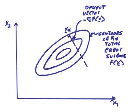
We will confine our attention here to descent algorithms. We first look at the total error surface
![]()
where g(x) is the computed forward
problem. The vector ![]() is the gradient of the
total error surface. This is a vector
which points in the direction of maximum ascent of the function F(x).
is the gradient of the
total error surface. This is a vector
which points in the direction of maximum ascent of the function F(x).
The gradient vector for a scalar temperature field point in the direction of maximum temperature change.
Ex) Direction of temperature gradient
Ex) The gradient vector for topography points in the direction of maximum ascent (perpendicular to contours of equal contours)
Now, linearize the forward problem as
![]()
where Ak is the sensitivity or Frechet derivative
operator ![]() . Then,
. Then,
![]()
![]()
where we have used a ![]() for simplicity. The gradient vector is then
for simplicity. The gradient vector is then ![]() and points in the direction
of maximum ascent. Let,
and points in the direction
of maximum ascent. Let,
![]()
where ![]() is the adjoint of Ak.
is the adjoint of Ak.
We want to construct a descent algorithm where at each iteration we move in the direction of maximum descent, thus
![]()
where ![]() is a scalar which
tells us how far to move. Thus,
is a scalar which
tells us how far to move. Thus,
![]()
We now have to find a way of picking ![]() .
.
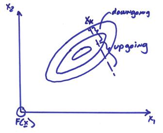
We want to pick ![]() so that we move along the
so that we move along the
![]() line until we reach a
minimum and are tangent to some contour of F(x). We thus want
line until we reach a
minimum and are tangent to some contour of F(x). We thus want ![]() , or
, or
![]()
where
![]()
![]()
Then,
![]()
This results in
![]()
![]()
![]()
Finally, we get

This algorithm is called the Steepest Descent algorithm. Note that in the nonlinear case, ![]() , where we have applied it to the stochastic inverse
objective function, can only be expected to be an approximation. . The
following steps are used
, where we have applied it to the stochastic inverse
objective function, can only be expected to be an approximation. . The
following steps are used
1) Compute Ak, the sensitivity
operator  , and also compute g(xk), the forward
problem. Hopefully this can be done in
the same step.
, and also compute g(xk), the forward
problem. Hopefully this can be done in
the same step.
2) Compute ![]() where
where ![]() is the adjoint and is easy
to compute given Ak.
is the adjoint and is easy
to compute given Ak.
3) Compute the scalar weight  . We may opt for an
approximate specification or computation of this scalar for nonlinear problems.
. We may opt for an
approximate specification or computation of this scalar for nonlinear problems.
4) ![]()
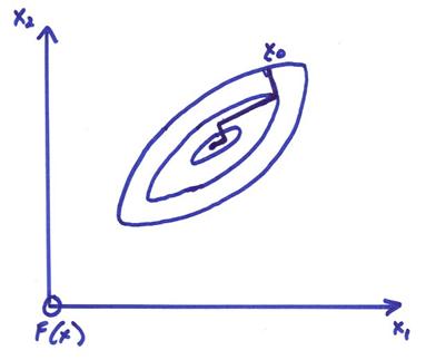
5) Repeat until ![]() is small. Thus in the descent approach, no inverses are
required. The figure below shows an
illustration of this where the contours of the objective function to be
minimized are shown as well as the iterative descent path to a minimum.
is small. Thus in the descent approach, no inverses are
required. The figure below shows an
illustration of this where the contours of the objective function to be
minimized are shown as well as the iterative descent path to a minimum.
One problem with this approach is that for highly elongated error surfaces (characterized by a wide spread of singular values for Ak), then many iterations may be required for convergence.
Convergence improvement can be obtained by using several techniques
1) Scaling the problem to reduce the spread of the singular values of Ak.
2) Use a modified descent algorithm called the conjugate gradient method.
Ex) Given y
and ![]() , as well as
, as well as ![]() , and
, and ![]() (no knowledge of the
range of x), then,
(no knowledge of the
range of x), then,
![]()
Let,
![]() , and
, and ![]()
then
![]()
and
 (Note
(Note ![]() cancels in the
combined term
cancels in the
combined term ![]() )
)
Let Ax = y be,

The solution to these equations is ![]() . Now let,
. Now let,
![]() .
.
The total error surface is then,
![]()
(Note the factor of ![]() added for simplicity
later), and
added for simplicity
later), and
![]()
Thus,
![]()
The gradient vector is then,
![]()
or
![]()
Now for our case,
![]()
![]()
and
![]()
For the first iteration of a descent algorithm,
![]()
![]()

The first iteration then gives
![]()
Further iterations would then be required to converge to the
solution ![]() .
.
We will
find that multiplying the data residual ![]() by the adjoint of the
sensitivity matrix is kinematically equivalent to seismic migration. An iterative sequence of seismic migrations then
results in a complete seismic inversion (Tarantola, 1984). For a complete seismic inversion, the ultimate
goal is to obtain
by the adjoint of the
sensitivity matrix is kinematically equivalent to seismic migration. An iterative sequence of seismic migrations then
results in a complete seismic inversion (Tarantola, 1984). For a complete seismic inversion, the ultimate
goal is to obtain  at each point in the
medium which would imply many unknowns and usually iterative methods would be
required.
at each point in the
medium which would imply many unknowns and usually iterative methods would be
required.
Conjugate Gradient
Method
The idea of
the conjugate gradient method is to modify the descent direction ![]() in order to reduce the
number of iterations required. The
process is then continued as before
in order to reduce the
number of iterations required. The
process is then continued as before
![]()
where now ![]() is a modified descent
vector and
is a modified descent
vector and ![]() is chosen to minimize
a line search in the direction
is chosen to minimize
a line search in the direction ![]() .
.
For
simplicity, lets just look at the linear problem g(xk) =
Axk and let ![]() with
with ![]() . Then, we will
minimize
. Then, we will
minimize
![]()
![]()
Letting Q = A*A and b = A*y where Q is a symmetric and positive definite matrix (all eigenvalues > 0), then
![]()
For a positive definite Q, a set of “Q-orthogonal” vectors p0,…,pN can be constructed
with a modified inner product such that ![]() , for
, for ![]() .
.
The vector x can be expanded in a generalized Fourier series in terms of p0,…,pN as,

where ![]() . But, we want
. But, we want ![]() or
or ![]() , and
, and ![]() . Then,
. Then,

For ,![]() , then
, then

where hk
is the grad vector ![]() above. Then, an iterative sequence can be
constructed as
above. Then, an iterative sequence can be
constructed as
![]()
where

Note that the pk are a “Q orthogonal” basis for the domain where
![]()
Note that this is just a modified Gram Schmidt procedure. For the linear case, it is guaranteed to converge to the correct answer in at most N iterations for an NxN Q matrix. All we need to do is be able to compute the “Q orthogonal” vectors pi.
In addition, the set of partial solutions, xk, k < N, minimize F(xk) not just on each line segment, but on the whole linear subspace spanned by p0,…,pk-1 (at least for a quadratic F(xk)). Thus, the gradient error vector hk is perpendicular to all pi, i = 0,k-1. Thus,
![]() for
for ![]()
This is a very useful property which allows us to compute the vectors pi from the gradient vectors hk.
The Conjugate
Gradient Algorithm
1) Choose ![]() . Move to
. Move to ![]() then
then ![]() .
.
2) The vector p1 must be in the space spanned by {h0,h1} and must be“Q orthogonal” to p0.
3) Continue this procedure to find other pk.
In other words, the vectors {p1,…,pk} are the Q orthogonal vectors {h1,…,hk}. This leads to the procedure,
For any ![]() , define
, define ![]() , then
, then

![]()

![]()
(where ![]() is the computed
gradient vector).
is the computed
gradient vector).
We
construct pk+1 such
that pk+1 is Q
orthogonal to pi, i = 0. … k, where
![]()
For i = k, the two terms cancel giving zero. For i < k, the second term is zero and the first term is zero since subspace [p0,…,pk]is also spanned by [h0,…,hk].
In summary, for a linear problem Qx = b for Q an (NxN) matrix, then we can solve this using several approaches.
1) Using matrix inversion, this can be solved in one step.
2) Using the steepest descent method, there will be a geometric error reduction at each step.
3) Using the conjugate gradient method, this will converge in at most N steps
Now for the more error surface for the stochastic problem, then
![]()
and
![]()
We can use this vector in the conjugate gradient algorithm
above. For the general nonlinear case,
it may not be necessary to compute ![]() exactly and some
approximations could be used.
exactly and some
approximations could be used.
The
convergence of a single step in descent algorithms is related to the spread of
the eigenvalues in ![]() . In the simplified
case, for
. In the simplified
case, for ![]() , then the convergence rate is proportional to
, then the convergence rate is proportional to  . Thus, we may want to
look for “preconditioner operators” for
. Thus, we may want to
look for “preconditioner operators” for
![]()
For example, let

If ![]() and
and ![]() are chosen
appropriately,
are chosen
appropriately, ![]() will have compressed
eigenvalues for
will have compressed
eigenvalues for ![]() with values near
unity. Preconditioner steps are
extremely important for the convergence speed of descent algorithms.
with values near
unity. Preconditioner steps are
extremely important for the convergence speed of descent algorithms.