EAS 657
Geophysical Inverse Theory
Robert L. Nowack
Lecture 13
Practical
considerations
I will cover briefly the following practical issues:
1) Log variables
2) Inequality/equality constraints
3) L1 norm
1) Log variables
In many cases, using ln (parameters) – ln (data) improves the inversion procedure.
Ex) For many physical problems the parameters can only have positive values and we must discriminate against negative parameter values.
Ex) There is generally a problem of units for different parameters and using log variables can address this.
Ex) In some cases, the data is complex (real and imaginary) and one wants to weight them appropriately.
As we saw earlier, methods that help to compress the range of singular values and eigenvalues will give better convergence. These issues can be dealt with by using a ln or log parameterization in both the data and the model parameters.
In our original linearized inversion scheme,
 (1)
(1)
The solution to (1) can be used to update the parameters as
![]()
With log parameters, we set up the linearized system as


or,
 (no
sum on i)
(no
sum on i)
Then,
![]()
or
![]()
a) Note that this procedure never allows xj to change sign.
b) Changing the units describing either the data or the parameters does not cause any changes in the equations.
c) In addition, complex data are dealt with using the definition of the log of complex numbers as,
![]()
Then,

and

Ex) Since high frequency seismic waves are of the form
![]()
where ![]() is the travel time, then
travel time inversions are log variable parameterizations using only the
imaginary part particular arrivals in the data.
is the travel time, then
travel time inversions are log variable parameterizations using only the
imaginary part particular arrivals in the data.

where the model parameters can be either velocity or slowness variables.
d) One other advantage of log parameterizations is the ability to deal with large parameter changes as one iterates using a linearized inversion scheme. Only one iteration may be needed if our parameters are off by an order of magnitude.
Ex) Consider the problem of finding x given tan (x). Of course, tan-1x is a standard function, but we will solve this by a linearized iteration, where
![]()
Now for a linear parameterization, ![]() , then
, then
![]()
or,
![]()
In log variables,

Then,

Let y = .01 (tan x = 0.01 where xtrue = 0.01 radians). Let’s start with x0 = 1.5 rad (a poor initial guess).
Now use both iterative procedures.
|
|
Linear Variables |
|
Log variables |
||
|
|
x |
y/tan x |
|
x |
y/tan x |
|
0 |
1.5 |
7.09 x 10⁻⁴ |
0 |
1.5 |
7.09 x 10⁻⁴ |
|
1 |
1.4295 |
1.42 x 10⁻³ |
1 |
1.0665 |
5.52 x 10⁻³ |
|
2 |
1.2903 |
2.88 x 10⁻³ |
2 |
.1356 |
7.33 x 10⁻² |
|
3 |
1.0250 |
6.07 x 10⁻² |
3 |
.0103 |
9.75 x 10⁻¹ |
|
4 |
.5840 |
1.51 x 10⁻² |
4 |
.01 |
1.0 |
|
5 |
.1310 |
7.59 x 10⁻² |
|
|
|
|
6 |
.0113 |
8.83 x 10⁻¹ |
|
|
|
|
7 |
.01 |
1.0 |
|
|
|
Thus, the log scheme makes about an order of magnitude improvement in the fit at each step while the linear scheme only improves the fit by about a factor of 2 at each step until near the end.
2a) Linear equality constraints (LEP)
Consider solving Ax = y in the least squares sense subject to s equality constraints Gx = h. These are hard constraints that we want to be satisfied exactly.
Ex) Assume a
constraint ![]() , or
, or 
Ex) Assume a
constrant ![]() , or
, or 
a) We could combine Ax = y with these equations, but this might lead to some roundoff errors, and we don’t know how large to make the relative damping. This also does not reduce the number of unknowns.
b) We could solve this by increasing the number of unknowns through “Lagrange multipliers”.
We want to
minimize ![]() with the constraints
with the constraints ![]() . This can be written
as
. This can be written
as
![]()
subject to ![]() . Now, there is no
solution if
. Now, there is no
solution if ![]() . Thus, we assume that
h lies in the range of G so
that a solution to the constraint equations exists.
. Thus, we assume that
h lies in the range of G so
that a solution to the constraint equations exists.
If P rows
of G are linearly independent, then the constraints remove P degrees of freedom
in the choice of x. Consider two feasible solutions x1, x2 that solve ![]() , then
, then
![]()
and
![]()
where N(G) is the nullspace of G.
Let ![]() and where
and where ![]() is any feasible
direction with respect to the linear equality constraints. Then,
is any feasible
direction with respect to the linear equality constraints. Then, ![]() .
.
In order to
examine the optimality of F(x)
about some xA along
a feasible direction ![]() , we examine the first order
, we examine the first order

For this to be a possible minimum, ![]() . This is a
constrained stationary point, and from this
. This is a
constrained stationary point, and from this ![]() must be perpendicular
to any feasible direction of the constraints.
Thus,
must be perpendicular
to any feasible direction of the constraints.
Thus, ![]() must be in the row
space of G or
must be in the row
space of G or ![]() for some vector
for some vector ![]() which are called the
Lagrange multipliers. These
which are called the
Lagrange multipliers. These ![]() are unique only if the
rows of G are linearly independent.
Thus, in order to construct an equivalent unconstrained problem, we must
solve
are unique only if the
rows of G are linearly independent.
Thus, in order to construct an equivalent unconstrained problem, we must
solve
![]()
and
![]()
for,
![]()
Then,
![]()
and
![]()
This can be written in matrix form as
![]()
where ![]() . This is an augmented
system which can then be solved for by any of the unconstratined ways that we
used previously.
. This is an augmented
system which can then be solved for by any of the unconstratined ways that we
used previously.
c) As an alternative approach, we can solve a reduced set of equations by using the SVD decomposition of G. Thus, using SVD,
![]()
and a general solution to the constraints is
![]()
where ![]() is an arbitrary N-P length vector assuming the
number of nonzero singular values of G is P.
Now substitute this into
is an arbitrary N-P length vector assuming the
number of nonzero singular values of G is P.
Now substitute this into ![]()
![]()
or,
![]()
which is now an unconstrained problem for the reduced vector
![]() .
.
Thus, we have three ways of solving constrained equality constraints problems
a) augmented equations (roundoff errors) – unknown vector has a length N
b) Lagrange multipliers – unknown vector has a length N+P
c) reduced set of equations (assumes we have explicit constraint equations) – unknown vector has a length N-P
2b) Linear inequality constraints (LIP)
Examples of linear inequality constraints include
Ex) nonnegativity constraints
Ex) range constraints on variables
1) Certainly the easiest way to introduce range constraints is to solve

which forces x to be “near” x0
for a small damping ![]() .
.
2) Minimize
![]()
subject
to ![]() . Note
. Note ![]() constraints are avoided
by using -1 as needed.
constraints are avoided
by using -1 as needed.
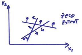
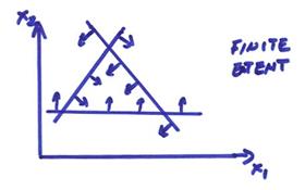
A lot of work has been done on this (mostly in books on optimization (see “Solving Least Squares Problems” by C. Lawson and R. Hanson (1995)). Each constraint defines a hyperplane that divides the space RN of solutions x in two, one in which the constraint is satisfied (the feasible half-space) and one in which the constraint is not satisfied (the infeasible half-space). The inequality constraints therefore define a volume in RN which might have zero, finite, or infinite extent.
Ex) A zero extent feasible space is shown below.
Ex) A finite extent feasible space is shown below.
Ex) An infinite extent feasible space is shown below.
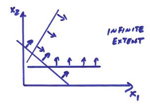
The volume has the shape of a polygon since for linear inequality constraints each equation is a plane. This polygon is convex like a football with no indentations.
We need to distinguish between
constraints that are active and inactive.
An inactive constraint does not restrict the perturbation of the
solution. An active constraint
does. Let ![]() be the set of active
constraints at some point x. Two such solutions can be written as
be the set of active
constraints at some point x. Two such solutions can be written as
![]()
![]()
where x1
– x2 = p, and x1 is a boundary perturbation. Any perturbation into the feasible space then
gives ![]() .
.
Consider a

For there to be a minimum, then
![]()
or ![]() must be in the column
space of G. Then,
must be in the column
space of G. Then,
![]() (similar to the equality
constraints case)
(similar to the equality
constraints case)
(Note, inactive constraints have zero Lagrange multipliers). However, since non-boundary perturbations are also feasible directions with respect to the inequality constraints, the point x will not be optimal if there exists any non-boundary perturbation that is a descent direction for F.
To take
this condition into account, we must have all ![]() . Thus, we have
. Thus, we have
![]()
![]()
![]() for the boundary
constraints
for the boundary
constraints
which is a variation of the Tucker-Kuhn conditions.
Thus, a
crucial distinction for the LIP case is the restriction on the sign of ![]() . A negative
. A negative ![]() would imply an infeasible
direction of descent. This is much more
complicated than the LEP problem since we don’t know which, if any, of the inequality
constraints hold. This must be solved
iteratively. Inequality constraints are
incorporated as equality constraints as necessary for solutions on the boundary.
would imply an infeasible
direction of descent. This is much more
complicated than the LEP problem since we don’t know which, if any, of the inequality
constraints hold. This must be solved
iteratively. Inequality constraints are
incorporated as equality constraints as necessary for solutions on the boundary.
For an interior solution,
![]()
For a solution on the boundary,

subject to ![]() . Lawson and Hanson (1995)
give an algorithm for least squares with inequality constraints as well as nonnegative
least squares or NNLS, (this is also available in MatLab).
. Lawson and Hanson (1995)
give an algorithm for least squares with inequality constraints as well as nonnegative
least squares or NNLS, (this is also available in MatLab).
3) Non-Gaussian statistics (the L1
norm)
In some cases there will be a few wildly scattered errors in the data. In general, these will cause least squares estimates to go haywire.
Ex) Take the average of M numbers
 where
where
 (2)
(2)
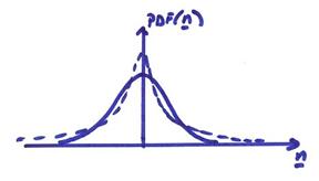
For the least squares solution, we assume that n is a set of Gaussian random variables with zero mean. A Gaussian PDf is shown by the solid line in the figure below.
By minimizing ![]() , we obtain
, we obtain  . Thus, the maximum
likelihood solution is just the “average value”. Let’s assume that M = 5
. Thus, the maximum
likelihood solution is just the “average value”. Let’s assume that M = 5

where 106 is some reading error. Then,
![]()
Thus, the least squares solution is hevily influenced by the single bad measurement. One way to avoid this is to take the “sample median”. The sample median is obtained by sorting yi from smallest to biggest and taking the middle value. In our case, ymedian = 1.0. Medians are much more robust to bad data points.
From a maximum likelihood point of view, use in equation (1) a modified PDf distribution for n. For example, let

This is an exponential distribution of the errors and has a much larger “tail” than the Gaussian distribution of errors has as shown by the dotted line in the figure above. This allows for the possibility of much larger excursions the errors. Maximizing this PDf is equivalent to minimizing the exponent. For Ax = y, we want to minimize,

Recall this is just the L1 norm for the length measure of the residuals. Hence, these minimizations are called L1 norm problems.
Ex) For the case above

or
![]()
where ![]() .
.
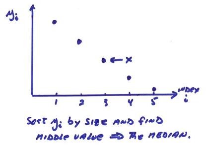
The solution to this is to sort yi from smallest to largest and then take the middle value. This is illustrated in the figure above and is the same as the sample median. The solution x results when we have as many points yi above as below in value, i.e. the middle value.
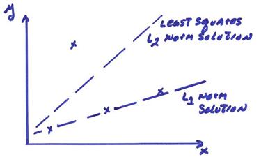
The equations for fitting a line are

The L1 norm solution to fitting a line finds two equations of the above M equations and solves these exactly to give the smallest absolute error for all the equations. This is illustrated in the figure below.
This can be done computationally by a modification of a well known algorithm called the simplex method originally used to solve linear inequality problems maximizing a linear objective function, linear programming.
The claim often made is that the L1 norm does what a human brain might do, it disregards points that are outliers.
For more details on robust data fitting using the L1 norm, see Claerbout and Muir (1973), (Robust modeling with erratic data, Geophysics, 826-844). A short, but effective, algorithm for the Ax = y problem solved using an L1 norm is given by Barrowdale and Roberts (1977), (Solution of an overdetermined system of equations in the L1 norm, Communications of the ACM, 17, 319-320).