EAS 657
Geophysical Inverse Theory
Robert L. Nowack
Lecture 14
Continuous Differential
Operators
We start by defining the inner product
![]()
where the bar above denotes the complex conjugate of the function. We now use the definition of the adjoint to provide a relation between A and A* (where A* is the adjoint operator). Thus,
![]()
First, we will discuss compatibility relations. Let
![]() then
then ![]() (1a)
(1a)
and,
![]() then
then ![]() (1b)
(1b)
Now from the relation for the adjoint, then
![]() (2)
(2)
since ![]() . This is called the
compatibility relation between the primary problem and the adjoint
problem. Thus, for all u and y satisfying equations (1a) and (1b), equation (2) must be
satisfied.
. This is called the
compatibility relation between the primary problem and the adjoint
problem. Thus, for all u and y satisfying equations (1a) and (1b), equation (2) must be
satisfied.
Ex) Let ![]() is in the null space
of A*, or from the adjoint theorems, y is in Rperp(A).
Then
is in the null space
of A*, or from the adjoint theorems, y is in Rperp(A).
Then ![]() , which is what y
being in Rperp(A) signifies.
, which is what y
being in Rperp(A) signifies.
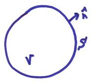
Before we go ahead and look at some Green’s functions, we need to define several adjoint operators. For differential operators, our inner products require the specification of boundary values on the volume of interest. Thus,
![]()
The volume v and its boundary S for a physical problem is shown below where
the outward normal of the boundary is ![]() .
.
The equation above can be used to derive A* and
the relevant boundary terms. The adjoint
operator A* is defined above to make an exact differential of the
term ![]() .
.
Ex)
Consider the ![]() in one dimension for
real functions, then
in one dimension for
real functions, then ![]() . Now,
. Now, ![]() where b.t. signifies the boundary term. From the definition of the adjoint,
where b.t. signifies the boundary term. From the definition of the adjoint,
Recall the formula for interpretation by parts,

In the adjoint formula above, let
![]()
and
![]()
then,
![]()
We see that
Thus, the adjoint A* makes the integrand of an
exact differential. Note that ![]() is not self adjoint since
A*
is not self adjoint since
A* ![]() A and also the
boundary term only equals zero if
A and also the
boundary term only equals zero if ![]() or
or ![]() , or a mixed combination.
, or a mixed combination.
Ex) In 3-D, this extends to ![]() ,
, ![]() , where
, where ![]() by the
by the
![]()
and the adjoint of the
![]()
Note, we will use the term Hermitian adjoint if all i’s are changed to –i’s in the adjoint.
Ex) A = C a constant. For this case, A* = ![]() and the b.t.
= 0.
and the b.t.
= 0.
Thus, A ![]() A* for a
complex number, but A = A* for a real number.
A* for a
complex number, but A = A* for a real number.
Ex)  in 1-D. For this case,

Use integration by parts in the form,
![]()
In the adjoint formula, let
![]()
and

then,
or
Thus,
and the adjoint can be written,

For this case,
![]()
Ex) 1-D wave operator (the Helmhotz equation)  with
with ![]() where v is the wave speed and
where v is the wave speed and ![]() is the frequency. Then,
is the frequency. Then,

where this is formally self adjoint.
Ex) 3-D Laplacian ![]()
Since the following equation is true
then,
As a summary, here are some adjoints for some simple differential operators (assuming a real inner product)
|
Au |
A*y |
Boundary Term |
|
|
|
|
|
|
|
|
|
|
|
|
|
|
|
|
where ![]() is the outward unit
normal on the boundary. For complex
inner products, then we need to change y
to
is the outward unit
normal on the boundary. For complex
inner products, then we need to change y
to ![]() in the boundary term.
in the boundary term.
Homogeneous boundary conditions occur when the boundary term is made to vanish by choosing the boundary conditions of the original problem and adjoint problem such that the boundary term is zero for the definition of the adjoint.
For the
moment, we won’t comment on inhomogeneous boundary conditions except to note
that we can always separate our problem ![]() into
into ![]() , where
, where

and

Let’s
return to the ![]() case with a special solution g when the source term
case with a special solution g when the source term ![]() , then
, then![]() . We can also define
solutions for the adjoint problem with
. We can also define
solutions for the adjoint problem with
![]() ,
,
where x is the receiver location and x1 is the source location. g(x,x1) is called the Green’s function for A and G(x,x1) is the Green’s function for A*.
Assume a complex inner product
![]()
and the definition of the adjoint as
![]()
where b.t. signifies the boundary terms. Then,
or,
![]() (3a)
(3a)
where ![]() is the complex
conjugate of the adjoint Green’s function for A*. For homogeneous boundary conditions, the
boundary term is zero. This can be interpreted
as finding u(x1) by putting a delta function source at each receiver
and evaluating at all interior points using G instead of g, where g is the
ordinary Green’s function for A.
is the complex
conjugate of the adjoint Green’s function for A*. For homogeneous boundary conditions, the
boundary term is zero. This can be interpreted
as finding u(x1) by putting a delta function source at each receiver
and evaluating at all interior points using G instead of g, where g is the
ordinary Green’s function for A.
Ex) For the ![]() operator, then
operator, then
 ,
,
assuming ![]() on the boundary. Note that assuming both u and
on the boundary. Note that assuming both u and ![]() on S raises questions of
incompatibility, which we will ignore for now.
on S raises questions of
incompatibility, which we will ignore for now.
Now let,
![]()
where g is the
ordinary Green’s function and x1
is the receiver location and x2
is the source location.. Now ![]() and from Eqn. (3a)
above for homogeneous boundary conditions where the boundary term is zero, then
and from Eqn. (3a)
above for homogeneous boundary conditions where the boundary term is zero, then
![]()
This is the general reciprocity relationship between the Green’s function for A and the adjoint Green’s function for A* where the bar signifies a complex conjugate. Thus, the ordinary Green’s function is related to the one for A* with the source and receiver interchanged and all i’s changed to -i’s.
Now for self-adjoint problems,
![]()
then,
![]()
which is the reciprocity relation for the self-adjoint case.
For the general case, the representation theorem above can also be written assuming homogeneous boundary conditions
![]() (3b)
(3b)
This form (3b) is often not as useful as (3a) since the sources
![]() in the medium could be
at many points, but there might be only one receiver position x1.
in the medium could be
at many points, but there might be only one receiver position x1.
Ex) As an alternative test to determine self
adjointness, one can look at the relation ![]() . As an example,
. As an example,
![]()
The Green’s function for ![]() is
is
![]() .
.
For this case,
![]() .
.
Thus, ![]() is self adjoint.
is self adjoint.
Ex)  is formally self
adjoint for the 1-D Helmholtz operator.
The Green’s function can be written as,
is formally self
adjoint for the 1-D Helmholtz operator.
The Green’s function can be written as,
![]()
Since,
![]()
But, the Helmholtz equation was shown earlier to be formally
self adjoint. This would imply that ![]() . Thus, from the
analysis of the Green’s functions, the Helmholtz equation is not strictly self
adjoint even though
. Thus, from the
analysis of the Green’s functions, the Helmholtz equation is not strictly self
adjoint even though ![]() .
.
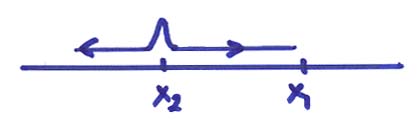
In the figure below, ![]() describes a wave
exploding from x2 to x1.
describes a wave
exploding from x2 to x1.
In the next figure, ![]() describes a wave imploding
from from x2 to x1.
describes a wave imploding
from from x2 to x1.
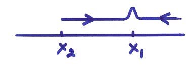
The sign of i shows that in the first case the source is exploding from x2 to x1 and in the adjoint case the source is imploding from x2 to x1.
Ex) For the acoustic wave equation

Fourier transforming this from time to frequency and then from position to wavenumber gives
and
![]()
For a medium with constant velocity c (this would be a homogeneous medium not to be confused with
homogeneous boundary conditions), then the Green’s function g can be written in different domains as
|
|
(x,t) Domain |
(x, |
(k, |
|
|
- sign is right going + sign is left going |
+ sign is right going - sign is left going |
|
|
|
where
- sign is out going |
For
|
|
|
|
- sign is out going + sign is in going |
+
sign is out going |
|


where ![]() is the Dirac delta
function,
is the Dirac delta
function, ![]() is the Heaviside step
function and the functions
is the Heaviside step
function and the functions ![]() and
and ![]() are Hankel
functions. For the wave equation in the
frequency and space domains, then
are Hankel
functions. For the wave equation in the
frequency and space domains, then ![]() , which is strictly not self adjoint, but still has spatial reciprocity.
, which is strictly not self adjoint, but still has spatial reciprocity.
Vector Green’s
Functions
Assume we have a function in three directions at each point x
![]()
For example, in a linear, elastic Earth, the wave equation in the frequency domain can be written as an operator A acting on a vector wavefield with the right hand side being the source field. The adjoint problem can be written in terms of the adjoint operator A*.

where u is the
wavefield for A and ![]() is the source field
for A, and
is the source field
for A, and ![]() is the wavefield for
A* and
is the wavefield for
A* and ![]() is the source field
for A* or
is the source field
for A* or
![]() and
and ![]()
We define the inner product ![]() to be
to be
and the adjoint is obtained from
assuming homogeneous boundary conditions.
From ![]() and
and ![]() , then
, then
 (4)
(4)
Let ![]() be a point force in the
“i” direction at position x1,
then
be a point force in the
“i” direction at position x1,
then
![]()
where j is the
receiver component, i is the source
direction, x is the receiver location
and x1 is the
source location. ![]() is the Kronecker delta
equal to 1 if i=j and zero otherwise.
is the Kronecker delta
equal to 1 if i=j and zero otherwise. ![]() is the Dirac delta
function which is only nonzero if x
= x1. Then,
is the Dirac delta
function which is only nonzero if x
= x1. Then,
 with homogeneous
B.C. (5)
with homogeneous
B.C. (5)
Now let,
![]()
then,
![]()
From equation (5), this results in the vector reciprocity relation,
![]()
General reciprocity then involves 1) interchange source and receiver locations, 2) interchange source orientation and receiver orientation, and 3) complex conjugate. For a self adjoint operator A* = A, then g = G and,
![]()
Note that the elastic wave equation in the frequency domain is not strictly self adjoint since for the homogeneous Green’s function
![]()
Applications to
Inverse Problems
Assume we are given a forward problem
![]() (6)
(6)
where this assumes the scalar wavefield u0(x)
and the source function ![]() . We would like to to
solve the following problems.
. We would like to to
solve the following problems.
I) The inverse source problem. What would the new wavefield be if we perturbed the source function? Then,
![]()
where, for example, the source might represent an earthquake
source. Since ![]() , then,
, then,
![]()
We can formally invert this equation using the Green’s function formalism as
![]() (7a)
(7a)
or
![]() (7b)
(7b)
by general reciprocity.
Note that for the scalar wave equation in the frequency domain (the
Helmholtz equation) ![]() and for this case
and for this case
![]() (7c)
(7c)
Note that this is in the form of a linear inverse problem
where the observed residual field ![]() is used to invert for
the source perturbation
is used to invert for
the source perturbation ![]() . Eqn. (7c) is often a
more useful form since
. Eqn. (7c) is often a
more useful form since ![]() implies putting a
source at each receiver point x1
and evaluating the field at all interior points x. Assuming the
number of receivers is small, this may be more computationally efficient in
terms of the number of forward problems required.
implies putting a
source at each receiver point x1
and evaluating the field at all interior points x. Assuming the
number of receivers is small, this may be more computationally efficient in
terms of the number of forward problems required.
II) The inverse medium problem. What would the new wavefield ![]() be if the operator A
is perturbed? This might result from
changing the velocity model incorporated in the operator A for the scalar wave
equation.
be if the operator A
is perturbed? This might result from
changing the velocity model incorporated in the operator A for the scalar wave
equation.
In the frequency domain, the scalar wave equation can be written in terms of the Helmholtz operator as

where v(x) is the medium velocity at all points x in the interior of the volume. Now,
 .
.
We want to solve,
![]()
where ![]() is the known source
and we know u0(x) for the unperturbed problem
is the known source
and we know u0(x) for the unperturbed problem
![]()
The perturbed problem can be expanded as
![]()
Since ![]() , this reduces to
, this reduces to
![]()
If we assume that ![]() are “small”, then as a
first approximation we can neglect the second order term
are “small”, then as a
first approximation we can neglect the second order term ![]() . Then, the linearized
problem for the perturbed wavefield can be written
. Then, the linearized
problem for the perturbed wavefield can be written
![]()
This is called the Born approximation. From the Green’s function formalism
![]() (7b¢)
(7b¢)
and
![]() (7c¢)
(7c¢)
where ![]() is the perturbed field
at the receiver xr and
is the perturbed field
at the receiver xr and
![]() is the original wavefield.
is the original wavefield.
For the Helmholtz operator, then

 .
.
Assuming

then,

Since for the scalar wave equation ![]() and assuming a point
source where
and assuming a point
source where
![]()
then
![]()
This reduces to,
 (8)
(8)
where ![]() can be interpreted as
the observed wavefield minus the calculated wavefield.
can be interpreted as
the observed wavefield minus the calculated wavefield. ![]() is the back
propagation from the receiver locations to the interior points in the model,
is the back
propagation from the receiver locations to the interior points in the model, ![]() is the propagation
from the sources to the interior model points and
is the propagation
from the sources to the interior model points and ![]() is the perturbed
velocity to be solved for. The figure
below illustrates the forward and back propagated fields for a buried target
zone in the Earth.
is the perturbed
velocity to be solved for. The figure
below illustrates the forward and back propagated fields for a buried target
zone in the Earth.
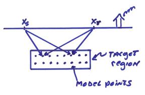
We would then have to do this for all sources and receivers to include all the data.
We know how
to solve this type of problem in the discrete case. Let ![]() , then
, then
![]()
where ![]() is the generalized
inverse. But, for the continuous case,
we need to investigate this further. It
is a linearized system for
is the generalized
inverse. But, for the continuous case,
we need to investigate this further. It
is a linearized system for ![]() given
given ![]() where
where
![]()
and
![]()
We now would like to see how this is related to what reflection seismologists call seismic imaging and migration.
From
equation (8), the sensitivity ![]() will only be “large”
when
will only be “large”
when ![]() and
and ![]() are in “phase”. This is sometimes referred to as an imaging
principle. The reflector exists when the
downgoing forward waves from the source coincide with the back propagated waves
from “pseudo” sources located at the receiver locations.
are in “phase”. This is sometimes referred to as an imaging
principle. The reflector exists when the
downgoing forward waves from the source coincide with the back propagated waves
from “pseudo” sources located at the receiver locations.
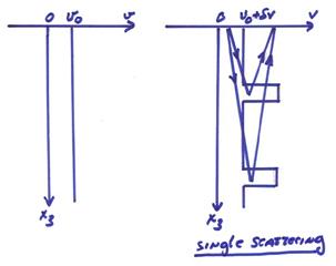
If ![]() is a constant, then
is a constant, then ![]() will be the Green’s
function for the homogeneous reference model. The Green’s functions in equation (8) contain
no “cross talk” in the perturbations. Hence
the Born approximation in equation (8) is a single scattering
approximation. It does not include
multiples scattering in the perturbations.
The figure below illustrates this.
will be the Green’s
function for the homogeneous reference model. The Green’s functions in equation (8) contain
no “cross talk” in the perturbations. Hence
the Born approximation in equation (8) is a single scattering
approximation. It does not include
multiples scattering in the perturbations.
The figure below illustrates this.
Seismic Imaging and Migration
There are a number of steps involved in seismic imaging. These include
1) Data collection. Seismic data is always collected in “common shot gathers”.
For multiple sources, the data can be regrouped into “common midpoint gathers”.
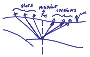
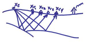
For a plane layered velocity structure, this would give one scattering point called the common depth point. This is a very logical way to organize the data. However, for laterally varying media, the scattering points will not be at the midpoint between shots and receivers. For a simple layer over a half space, this is illustrated below.
In this case, the scattering points are all at the midpoint, where h is the half offset between the shot and receiver and xM is the midpoint location.
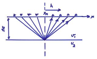
2) Normal Moveout and Stack
First, we need to organize the data into common midpoint (CMP) gathers at each midpoint location xM.
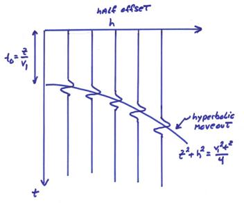
In order to obtain a representative reflection trace for that midpoint position, one can perform a “normal” moveout to align the arrivals and stack. This is called a CMP stack.
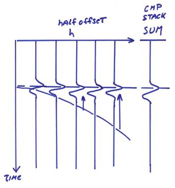
If the average velocity v1
to the reflector is chosen correctly for the normal moveout correction, this stacking
operation will give a large increase in coherent signal to noise. A ![]() increase in signal to
noise is possible, where N is the number of traces stacked (all “statics” due
to a near the surface weathering zone, topography, and lateral velocity
variations must be removed in order to get the full benefit of the stack).
increase in signal to
noise is possible, where N is the number of traces stacked (all “statics” due
to a near the surface weathering zone, topography, and lateral velocity
variations must be removed in order to get the full benefit of the stack).
3) Plot all the CMP stacked traces at the midpoint positions xM. This results in a zero offset stacked seismic section in (x,t) and is illustrated below.
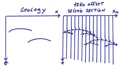
Of course we would need to stack the data to obtain the effective zero offset section. Alternatively, we could just plot a near offset trace (or any fixed offset trace at xM) if we choose not to stack, but this would not have the noise cancellation benefits of the stack This entire procedure can be viewed as a partial solution to the inverse problem since a blurred version of the “reflected” parts of the data is displayed.
The zero offset section can be viewed as an ensemble of experiments performed using a moving zero-offset source-receiver pair at each position along the surface x.
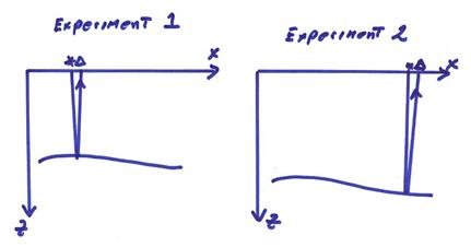
Naturally, this type of reflection or echo experiment will be most sensitive to abrupt changes in the velocity.
Since for normal incidence the reflection coefficient is proportional to
![]() ,
,
we will be inverting for the seismic reflectivity R and from
this estimating changes in the impedance I which is the combined variable![]() times v. At the outset, we will assume that the smooth
variations in velocity are known (say
times v. At the outset, we will assume that the smooth
variations in velocity are known (say ![]() or a constant v0). We need this in any case to take advantage of
the stack, but we could again have used just a near offset trace to get a
non-stacked common offset section. To
obtain the smooth part of the velocity model, velocity analysis can be
performed by maximizing the semblance or power in the stack for different trial
velocity models
or a constant v0). We need this in any case to take advantage of
the stack, but we could again have used just a near offset trace to get a
non-stacked common offset section. To
obtain the smooth part of the velocity model, velocity analysis can be
performed by maximizing the semblance or power in the stack for different trial
velocity models ![]() .
.
We now want to investigate abrupt changes in the velocity giving rise to reflections. Thus, we separate the velocity model into a slowly varying background velocity and a fast varying reflectivity.
Now, what would the reflectivity response be to a small point scatter in the earth? Assume initially a homogeneous background velocity model. Also, assume a zero offset source receiver pair moving along the surface. As shown in the figure below, a set of diffracted arrivals can be obtained from the multiple source-receiver pairs.
The 3-D point source response in the time domain is,

The received signal will then be
![]()
where D is a diffraction coefficient related to the perturbation![]() , the point reflectivity, and * signifies convolution. Then,
, the point reflectivity, and * signifies convolution. Then,
![]()
If we are just interested in timing (ignoring amplitudes), then we could consider our multiple experiment replaced by one experiment with a source placed at the scattering point in the earth and all velocities changed to (v/2).
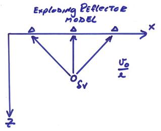
This has an incorrect amplitude, but the correct timing, and is called the “exploding reflector model”. The simultaneous exploding of multiple scatterers in the subsurface is illustrated below.
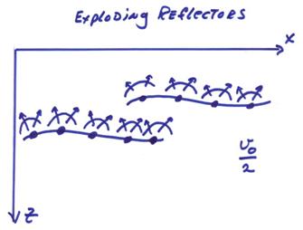
Thus, we replace many numerical experiments by one experiment where all reflectors are made up of point scatterers that “explode” at t = 0.
Now let’s look alternatively in the (x,t) domain. The figure below shows one pulse originating from a semicircle of scatterers with pulses all arriving at the same time.
A semicircle of point reflectors would give one pulse in the
(x-t) zero offset section at time ![]() and location
and location ![]() .
.
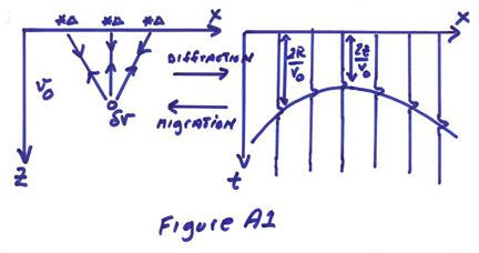
We thus have two ways of converting a zero offset section into an approximate model of the reflectivity in (x,z).
1) Assuming an average velocity v, sum hyperbolas on the (x-t)
record sections and put the energy in (x,z) at the point ![]() (Figure A1).
(Figure A1).
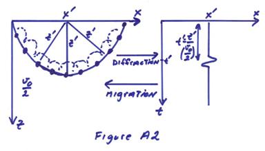
2) Take each point in the (x,t) record section and
smear this energy out into semicircles in (x,z) of equal amplitude and put it at center
![]() with radius
with radius ![]() (Figure A2).
(Figure A2).
Either of these procedures is known as Kirchhoff migration
in the time domain. A commercial diffraction
stack algorithm would typically work on the transformed (x,![]() ) section in the frequency domain and do the equivalent
operation. Note that if
) section in the frequency domain and do the equivalent
operation. Note that if ![]() constant, then ray
tracing must be performed to find the times to the point diffractors in the
subsurface. A major problem occurs in
complicated geologic structures where we don’t know either the reflectivity D(x,z)
and the smooth velocity v(x,z). There are errors in both determinations and
possible tradeoffs.
constant, then ray
tracing must be performed to find the times to the point diffractors in the
subsurface. A major problem occurs in
complicated geologic structures where we don’t know either the reflectivity D(x,z)
and the smooth velocity v(x,z). There are errors in both determinations and
possible tradeoffs.
A reference for Kirchhoff migration is: Schneider (1978), Integral formulation for migration in two and three dimensions, Geophysics, v. 43, p. 49-76.
The figure
below shows an example of a CMP stacked section above and a migrated seismic
section below. The seismic line is 11 km
long across the

Born Inversion
To investigate seismic migration as an inverse problem, we will start with the scalar wave equation

where u(t,x)
is pressure field in t and x, ![]() (t,x) is the source, and
(t,x) is the source, and ![]() is the spatially varying
velocity. In the frequency domain, the
wave operator is
is the spatially varying
velocity. In the frequency domain, the
wave operator is

Assuming homogeneous B.C. and the ordinary Green’s function, then
![]()
The initial forward problem for operator A0 can be written
![]()
and we want to find the new field such that

Assume that the source is known and
![]() , then
, then
![]()
or
![]()
Then, with ![]()
![]()
This is an exact equation for ![]() . If
. If ![]() is a small and second
order, then we can neglect it resulting in
is a small and second
order, then we can neglect it resulting in
![]()
This is called the Born approximation. For our case,

From the Green’s function formalism
![]()
and from the special reciprocity for the wave equation, then
![]()
In a homogeneous medium, the Green’s function can be written in the frequency domain as

For a point source at xs
and a source time function spectra ![]() , then
, then

The perturbed pressure field can then be written as,
 (9)
(9)
Eqn. (9) is the linearized Born approximation for the
perturbed field for a slight perturbation in the velocity ![]() . Thus
. Thus ![]() + scattered waves from
+ scattered waves from
![]() + scattered waves from
+ scattered waves from
![]() + … . This is also called the single scattering
approximation. In doing this, we have
left out all the “cross talk” between
+ … . This is also called the single scattering
approximation. In doing this, we have
left out all the “cross talk” between ![]() and
and ![]() . This “crosstalk” is
called multiple scattering in the perturbations and is included in the
. This “crosstalk” is
called multiple scattering in the perturbations and is included in the ![]() term which we left
out.
term which we left
out.
Considering only the linearized approximation
![]()
where B is the linearized Born operator.
The inverse
Born problem is to find ![]() from
from ![]() . Thus, symbolically
we can write the solution as
. Thus, symbolically
we can write the solution as
![]()
We would be finished except that most inverse operators are hard to find. But, adjoint operators are usually easy to find. Inverse operators can also be constructed from adjoint operators. The adjoint operator B* takes us from the data space to the model space.
For the overdetermined case, ![]()
For the underdetermined case, ![]()
Since B is only an
approximate, linearized sensitivity operator, we may not need to know ![]() exactly. Thus, let
exactly. Thus, let
![]()
where ![]() is the observed
wavefield at the receivers minus the calculated wavefield in the initial
velocity model and
is the observed
wavefield at the receivers minus the calculated wavefield in the initial
velocity model and ![]() is a small number. Now define B* from
is a small number. Now define B* from
![]()
where ![]() is the inner problem
over sources, receivers, and frequency.
is the inner problem
over sources, receivers, and frequency.
Define the inner products as
![]()
and
Now from the definition of adjoints above
![]() ,
,
since velocity is defined with a real inner product. Then,
![]()
and
![]()
Now,
then,
![]()
Then,
 .
.
For coincident sources and receivers,
Now, this can be transformed into the time domain where we use the following identities where F.T. denotes the Fourier Transform.
![]()
![]()
![]()
Let,
![]()
Now,
![]()
where “*” signifies convolution. This gives,
This reduces to
 (10a)
(10a)
with
![]() (10b)
(10b)
Eqn. (10b) is the
cross correlation with the second derivative of the source time function. Eqn. (10a) says to sum energy along
hyperbolas weighted by  . This is not quite
the same as the empirically derived Kirchhoff formula, but we haven’t accounted
for (B*B)-1 as yet.
. This is not quite
the same as the empirically derived Kirchhoff formula, but we haven’t accounted
for (B*B)-1 as yet.
Thus, the action of adjoint B* is equivalent to a matched filter operation with the source function plus a Kirchhoff style summation.
A complete velocity inversion could be posed in terms of an iterative sequence of Kirchhoff migrations. This approach was described by Tarantola (1987). An approximate (B*B)-1 compensates for the amplitude part to give a modified amplitude term.
More complete discussions of Born inversion of seismic reflection data are described below.
Bleistein, N., K. Cohen, and F. Hagin (1987). Two and one half dimensional inversion with an arbitrary reference, Geophysics, 52, 26-36.
Bleistein,
N., K. Cohen, and J. Stockwell (2001).
Mathematics of Multichannel Seismic Imaging Migration and Inversion,
Springer,
Jin, S., R. Madariaga, J. Virieux, and G. Lambare (1992). Two-dimensional asymptotic iterative elastic inversion, Geophys. J. Int., 108, 575-588.
Tarantola,
A. (1987). Inverse Problem Theory,
Elsevier.