EAS 657
Geophysical Inverse Theory
Robert L. Nowack
Lecture 15
One-Dimensional Media
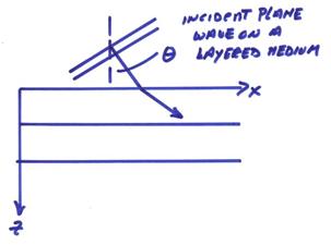
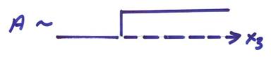
A special type of earth structure which occupies a primary interest of geophysicists are structures that vary in one-dimension only. An example is shown below varying in z or x3 only.
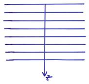
These can be layers or continuous functions of z, for example, c(z), ![]() .
.
Ex) In exploration seismology, a borehole sonic log may be given. A synthetic zero offset seismogram can then be calculated, including all internal reverberations, for that structure.
The figure below shows velocities with depth from a sonic log directly measured down a borehole, seismic rays from a surface source and receiver, and a synthetic seismogram.
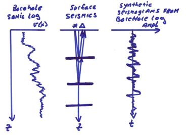
The synthetic seismograms from the borehole log can then be compared with an observed surface seismic trace.
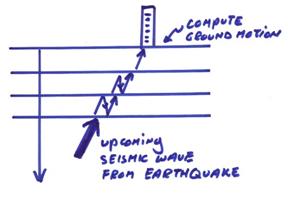
Ex) In earthquake seismology, assuming a layered soil column under a large building, the seismic displacements and accelerations at the base of the building may be needed given upcoming seismic waves from an earthquake.
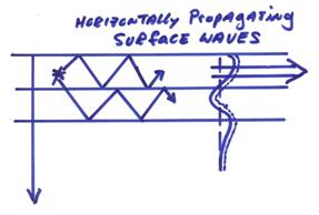
Ex) Surface waves in earthquake seismology or “ground roll” in reflection seismology can be thought of as a multiple reverberating set of seismic waves propagating horizontally in a near surface layering.
By using separation of variables for 1-D media, closed form expressions for reverberating waves can be found (instead of tracking many rays!).
First note that since a general curved initial wavefront can be decomposed into a set of plane waves, we will look only at an incident plane wave for a 2-D (x1,x3) case with c = c(x3). Thus, the medium is 1-D, but the propagating wave can be 2-D or 3-D.
An example of a tilted plane wave incident on a layered media.
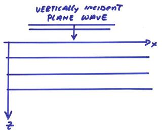
To simplify the problem even further, we will investigate only normally incident plane waves on a layered media.
For this case, forward modeling exact expressions and exact inverse expressions can be derived for the sonic log case.
1) Sonic log velocity structure ![]() synthetic seismic
waveform
synthetic seismic
waveform
for a surface
source
2) Observed seismic waveform ![]() infer the
velocity structure
infer the
velocity structure
for a surface source
We will first investigate the forward problem for the calculation of the reverberatory waves in the structure. We will illustrate the process using the acoustic wave equation in 1-D starting with the following physics.
1) The gradient of the pressure P gives rise to an acceleration in the mass density related to the inertial term as
![]() (1a)
(1a)
and
![]() (1b)
(1b)
where ![]() are the components of
the particle velocity in the x1
and x3 directions,
respectively, and
are the components of
the particle velocity in the x1
and x3 directions,
respectively, and ![]() is the density.
is the density.
2) The divergence of the particle velocity times the incompressibility K equals the rate of pressure decrease
 (2)
(2)
where S(x1,x3,t) is a pressure source.
Note that the pressure rate ![]() is related to the
dilatation rate
is related to the
dilatation rate ![]() by
by
![]()
where ![]() and u is the displacement field. Then,
and u is the displacement field. Then,
![]()
This is equivalent to Eqn. (2) without the source term. Equations (1) and (2) can be written in several different ways. In terms of first order equations
 (3a)
(3a)
where K is the bulk modulus.
Most physical systems can be described in terms of first order matrix systems by introducing new variables. Thus,
![]()
Alternatively, we could write Eqn. (3a) in terms of the pressure P alone by writing this as a second order system. Taking the second derivative of equation (2)

From Eqn. (1)

If density is approximately constant, then
 (3b)
(3b)
where
![]()
This is the general scalar wave equation.
Note, that in doing this we have lost the separation of ![]() and K.
We will often prefer to work with first order equations (3a) whenever
possible.
and K.
We will often prefer to work with first order equations (3a) whenever
possible.
Ex) Heat flow in the x1-x3 plane. The heat flow H can be written as
![]()
![]()
where ![]() is the thermal
conductivity and T is the temperature.
Also,
is the thermal
conductivity and T is the temperature.
Also,

where C is the heat capacity, and s is a heat source. These equations can be combined as,

which is a diffusion equation for the temperature field T(t,x1,x3).
If we have
a 1-D acoustic media, then ![]() ,
, ![]() which are not functions
of either t or x1. We can then use
Fourier transforms to reduce the Eqns. (3a) using
which are not functions
of either t or x1. We can then use
Fourier transforms to reduce the Eqns. (3a) using
Then Eqn. (3a) becomes,

From the first two equations,
![]()
![]()
From the third equation,
![]()
or

resulting in

V1 then becomes an auxiliary variable and the system can be reduced to two equations.

We thus no longer have partial derivatives in the matrix and this is of the form
![]() (4)
(4)
which is an initial value problem
given S and X = X(![]() ) where
) where  . To find the pressure
field in the time and space domain at some depth x3, then
. To find the pressure
field in the time and space domain at some depth x3, then
and the same for ![]() .
.
Let’s first
comment on Eqn. (4) in terms of degree of
singularity. Assume we have a welded
interface with a step change in K and ![]() . Then the
matrix A has a step discontinuity in its coefficients. This is illustrated below.
. Then the
matrix A has a step discontinuity in its coefficients. This is illustrated below.
In a source free region, ![]() . Now in order
for this equation to have balanced orders of singularity, then
X can, at most, have a discontinuity in the x3
derivative and, therefore, must be continuous in x3 which is illustrated below.
. Now in order
for this equation to have balanced orders of singularity, then
X can, at most, have a discontinuity in the x3
derivative and, therefore, must be continuous in x3 which is illustrated below.
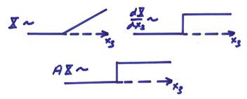
Thus, in a source free region, the field is always smoother than the material parameters.
Numerical Matrizants (propagators)
Starting with Eqn. (4), then taking a finite difference
![]()
or
![]()
This can be used recursively to find X(x3) for any ![]() . Let
. Let ![]() . Then for each
interval in depth where
. Then for each
interval in depth where ![]() , then
, then
![]()
which is a recursion relation. Given X0 at depth
![]() , then
, then
![]()
![]()
![]()
![]()
![]()
Thus, we can find ![]() at a bottom depth from
at a bottom depth from
![]() at a top depth as,
at a top depth as,
![]()
Since this is a 2x2 matrix equation, we have two equations for
four unknowns being the components of ![]() and
and ![]() . Thus, we need
two additional boundary conditions to determine the problem which we discuss later.
. Thus, we need
two additional boundary conditions to determine the problem which we discuss later.
M is called a numerical matrizant or propagator. If parts of the medium have constant material parameters and contain no sources, then
![]()
By analogy to the scalar case where ![]() . For the
matrix case, we can write
. For the
matrix case, we can write
![]()
We will interpret the exponential
of a matrix in terms of its
![]()
or to first order
![]()
Thus, the finite difference approximation above to the original equation gives the first two terms of the exact homogeneous solution.
We now will interpret ![]() in terms of up and
down going waves so we can get the two remaining boundary conditions.
in terms of up and
down going waves so we can get the two remaining boundary conditions.
The transformed acoustic wave equation can be written as

where

This is again of the form
![]()
where in a source free region, this can be written as
![]()
We now want to transform A into an equivalent diagonal form. First, we find the eigenvalues of A

then,
![]()
and
![]() which are the imaginary
eigenvalues
which are the imaginary
eigenvalues
Let,

then,

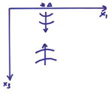
The vertical component of the wavenumber vector k3 is from the figure below
![]()
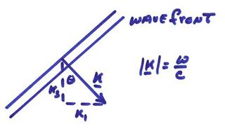
and
![]()
We now need to find the eigenvectors where
![]()
The two eigenvectors can be put into one equation as

For our case,

then,

For the two eigenvalues ![]() and
and ![]() , the eigenvectors, and X1 and X2
as
, the eigenvectors, and X1 and X2
as

Then,

We will leave these eigenvectors unnormalized so that our physical interpretation of up and down going pressure waves have the right units.
In terms of matrices, the eigenvalue problem can be written as
![]()
where ![]() is a diagonal matrix
with the eigenvalues along the diagonal. Then,
is a diagonal matrix
with the eigenvalues along the diagonal. Then,

or
![]()
with

Note that,

where
![]()
Thus,

Finally,
![]()
I is called the vertical acoustic impedance which is also the ratio of the pressure to the vertical particle velocity. One over the acoustic impedance is called the acoustic admittance. Then,

Now return to the general equation
![]()
In a source free, homogeneous medium,

where P is the Fourier transformed pressure
and V3 is the vertical particle velocity. Let ![]() in a homogeneous
region, then
in a homogeneous
region, then
![]()
Let ![]() , then
, then
![]() (5)
(5)
in a source free, constant medium. Let,
![]()
where we will interpret U and D to be up and down going waves. Then,

If ![]() are up and down going
waves, then
are up and down going
waves, then
![]()
![]()
The solution to Y(x3) in Equation (5) is

Using a ![]() , then
, then

But,  , then

Thus, U(x3) and D(x3) in a homogeneous medium are indeed in the form of up and downgoing waves.
If we return to the original problem

this has a solution ![]() where
where ![]() . Recall Sylvester’s
theorem, which states that the function of a square matrix with a complete set
of eigenvectors can be written as
. Recall Sylvester’s
theorem, which states that the function of a square matrix with a complete set
of eigenvectors can be written as ![]() which can be derived using
a
which can be derived using
a
 (6)
(6)
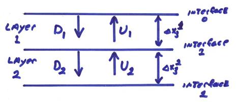
Since the pressure and vertical particle velocity are
continuous across a material discontinuity, we can use Eqn.
(6) to relate ![]() at the top of layer 1
to the top of layer 2 (see figure below).
at the top of layer 1
to the top of layer 2 (see figure below).

since,

Then,

where,

with ![]() and
and ![]() . This can be written
. This can be written

or

Then,  with
with

where ri is the acoustic reflection coefficient. The acoustic transmission coefficient is

Then,

The recursion of up and downgoing waves from the top of the stack of layers to the bottom is
 (7)
(7)
This is illustrated in the figure below.
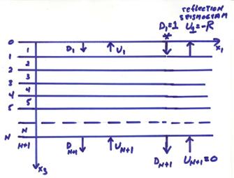
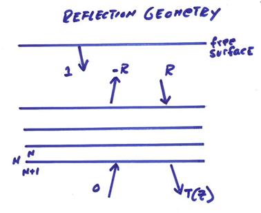
For the reflection seismology case with a source at the top and no waves coming from below, then (neglecting the free surface)
![]() source
source
![]() reflection seismogram
reflection seismogram
![]() transmission
seismogram
transmission
seismogram
![]() no waves from below
no waves from below
From Eqn. (7) and now including the free surface, then

where ![]() . From the
first equation
. From the
first equation
![]()
or
![]()
In the time domain, ![]() corresponds to
corresponds to ![]() in the frequency
domain. The Z variable above is
in the frequency
domain. The Z variable above is
![]()
which is related to the two-way time through layer i. Thus, the inverse transform of R(Z) will give the reflection seismogram with reflection delayed in time. This will work for any inclined plane wave incidence on the stack of layers. In order to do this, we need to first solve the layer matrix Eqn. (7) above with the boundary conditions to give R(Z) and T(Z).
We will now set up the inverse problem in a discrete layered model from a physical point of view.
Inversion of a
What can we recover about the Earth from a normal incident
reflection seismogram? We will look just
at a 1-D medium where ![]() . Assume a
discrete stack of layers each with a constant
. Assume a
discrete stack of layers each with a constant ![]() .
.
A Goupillard medium [Goupillard (1961), Geophysics 26, 754-760] is designed to have constant travel-times in all layers.
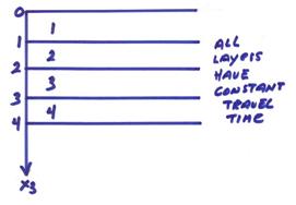
In each layer

Then, for the up and down going pressure waves,

We will construct the layers so that

Thus the thicknesses change in such a way that all the ![]() ’s are constant.
We could also make the layers arbitrarily thin to approximate the continuous
case. Suppose we have an impulsive
source at the surface as illustrated below.
’s are constant.
We could also make the layers arbitrarily thin to approximate the continuous
case. Suppose we have an impulsive
source at the surface as illustrated below.
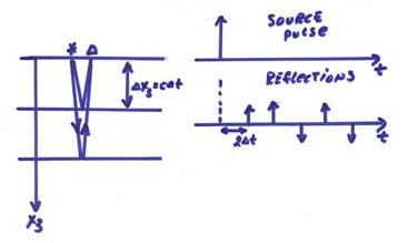
We record at the surface a set of equally spaced impulses, thus
![]()
where R(t) is the reflection seismogram. Transforming this seismogram to the frequency domain gives
Since ![]() corresponds to
corresponds to ![]() in the frequency
domain, then
in the frequency
domain, then
![]()
Define ![]() . Then the
reflection seismogram in the frequency domain is
. Then the
reflection seismogram in the frequency domain is
![]()
This is a power series in Z called a Z-transform. It is related to a Fourier transform for a sampled signal.
IMPORTANT: The values an in the time domain are the coefficients of Zn, where Zn is a time shift operator in the frequency domain. Thus, Z is related to the two way travel time in each layer. (Note that Z-transforms are very popular in geophysics, as well as engineering.)
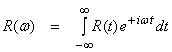
Let’s look
at an incident pulse with unit amplitude  incident on a
particular interface. For
an incident pulse from above.
This can be shown as
incident on a
particular interface. For
an incident pulse from above.
This can be shown as
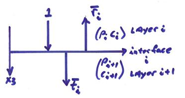
For an incident pulse from below, then
We require at the boundary, continuity of pressure P and vertical
particle velocity ![]()
1) ![]()
2) ![]()
We can define up and down going waves in terms of either pressure or vertical particle velocity. Note, for seismics, we will use displacement waves (a vector quantity) and for acoustics, we will use pressure (a scalar quantity).
From condition 1) for pressure waves
![]()
where ri is pressure reflection coefficient and ti is the transmission coefficient, and also
![]()
where
![]()
The relation between ![]() and
and ![]() is
is
![]()
Thus, if we know any one of the quantities
![]() , we can determine all of them.
, we can determine all of them.
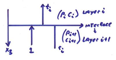
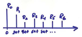
Now we
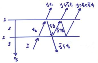
apply an impulse with unit amplitude at the surface of a stack of layers. A scattering diagram is shown below where x3 is the horizontal axis and
time is the vertical axis. The discrete
reflection seismogram has amplitudes recorded every ![]() time intervals.
time intervals.
The following layers stripping approach can be used to find the reflection coefficients.
1) From the first amplitude observation in time at
![]() on the reflection seismogram, we can obtain
on the reflection seismogram, we can obtain
![]() .
.
2) We can then determine ![]() .
.
3) It is assumed we know ![]() .
.
4) From the second amplitude observation at time ![]() , get
, get ![]() and from this, obtain
and from this, obtain ![]() .
.
Continuing in a recursive manner, we can obtain ![]() from the amplitudes at
from the amplitudes at
![]() times on the
reflection seismogram. From the
reflection coefficients, we can then obtain
times on the
reflection seismogram. From the
reflection coefficients, we can then obtain ![]() .
.
Thus, we can use this approach to obtain the seismic impedances
Ii from the observed reflection
seismogram. Note this is for vertical
incidence only. Unless we know ![]() , we can’t find ci separately. The specific formulas for both the forward
and inverse case will be given later, but this is the general approach.
, we can’t find ci separately. The specific formulas for both the forward
and inverse case will be given later, but this is the general approach.
Let’s now look at a simple layer resonance
The transmitted wave above interface 1 has the form
![]()
where ![]() corresponds to the layer
time delay operator. The transmitted
wave can be written in a closed form as,
corresponds to the layer
time delay operator. The transmitted
wave can be written in a closed form as,
![]()
This is an exact expression for the entire infinite set of reverberations in the layer. We would like to do this to obtain the exact expression for a set of layers.
For the discrete case,
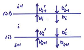
The primes denote motions at the bottom of each layer. From this,
![]()
![]()
or
![]()
![]()
and

This can be written as

Since ![]() , then
, then
![]()
![]()
and


![]() Then,
Then,

Since ![]() is the operational
two-way travel time operator in the layer, multiplying by
is the operational
two-way travel time operator in the layer, multiplying by ![]() is equivalent to
delaying the wave by the layer thickness time
is equivalent to
delaying the wave by the layer thickness time ![]() . Then,
. Then,

where
 is equivalent to the layer
matrix found in the earlier analysis.
Now,
is equivalent to the layer
matrix found in the earlier analysis.
Now,


or in general
 (8)
(8)
where
![]()
![]()
This can be shown by adding next term and showing it has the same form.
Equation (8) has the same form as equation (7) in the earlier analysis.
Now introduce the reflection seismogram,
![]()
where Z is the unit delay operator.
The transmission seismogram can also be written as,
![]()
where we have a reflection geometry with a source above and no sources at the bottom as shown in the figure below.
Thus,

and

Then,
From the first equation,

where
![]()
with
![]()
The transmission seismogram can be manipulated into the form
Thus, for the forward problem, we can calculate both R(Z) and T(Z) in the reflection geometry.
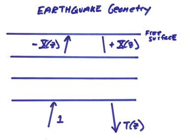
We could also set up the problem in the earthquake geometry (for this case in the acoustic case, but also in the elastic case) as shown in the figure below.
For the
inverse reflection problem, we want to get the reflection coefficients ![]() from the reflection seismogram
from the reflection seismogram ![]() . From
. From
![]()
and
![]()
Now,

and

where R(Z-1) is a change in the order of time. This equals
![]()
Now ![]() , and
, and
![]()
![]()
and,
![]()
where ![]() is proportional to the
determinant of the propagator except for a
is proportional to the
determinant of the propagator except for a  factor.
Now, the determinant of a product of matrices is the product of the determinants. Thus,

then,

where ![]() is causal with no
negative powers in Z. This simple fact
is enough to determine the reflection coefficients from the waves. Thus, all negative powers of z must vanish!
is causal with no
negative powers in Z. This simple fact
is enough to determine the reflection coefficients from the waves. Thus, all negative powers of z must vanish!
![]()
![]()
![]()
![]()
![]()
From causality then, all these terms up to Z-N must vanish. This results in a matrix equation

where the matrix is a Toeplitz matrix. If
we are given ![]() , this system of equations can be used to recursively
solve to find the reflection coefficients.
The impedances can be found from the estimated reflection coefficients
, this system of equations can be used to recursively
solve to find the reflection coefficients.
The impedances can be found from the estimated reflection coefficients ![]() .
.
This is a more formal approach to the qualitative approach given before for the inversion of a reflection seismogram. For more details on this approach, see Claerbout (1976) (Fundamentals of Geophysical Data Processing, McGraw-Hill), and Aki and Richards (1980) (Quantitative Seismology, Freeman).