EAS 657
Geophysical Inverse Theory
Robert L. Nowack
Lecture 4a
Solutions of Linear
Mapping
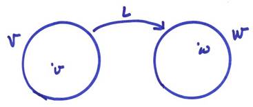
Consider the matrix equation
Lv = w
where given w, we want to find v.
The possibilities include
1) A unique solution exists to Lv = w
2) A solution exists, but it is not unique
(i.e., many v satisfy Lv = w)
3) No solution exists and we want the best
approximation (Lv ![]() w).
w).
We will find that

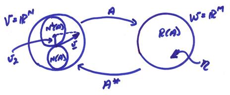
Let
V = N(L) + Nperp(L) with the solution to Lv
= w as
v = v1 + v2
where
v1 ![]() N(L)
N(L)
v2 ![]() Nperp(L)
Nperp(L)
Claim: v2 is always unique. To show this, assume
![]()
but we’ve assumed
![]()
Define the minimum length solution v as the solution where || v1 || = 0.
For
case 3), no solution exists, but we want the best approximation solution of w
which lies in the range of L. Thus, if Lv ![]() w, then given w,
minimize || Lv1 – w ||2.
w, then given w,
minimize || Lv1 – w ||2.
Define
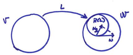
W = R(L) + Rperp(L) and w
= w1 + w2, with w1 ![]() R(L) and w2
R(L) and w2 ![]() Rperp(L), where
Lv = w1. The
resulting solution for the case 3) can be either unique or nonunique.
Rperp(L), where
Lv = w1. The
resulting solution for the case 3) can be either unique or nonunique.
Adjoint
Transformation, L*
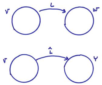
If L is a mapping from v to w, let L* be a mapping from w to v.
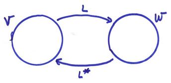
L: v ![]() w
w
L*: w ![]() v
v
Note that L* is not L-1. Thus, even if L is not onto W, L* is still defined over W.
Assume an inner product is defined in both V and W. Then the adjoint is defined such that
![]()
Ex) For real matrices, A* = AT, the transpose.
Properties of L*
1) L* always exists
2) L* is unique
3) If L is linear, then L* is linear
4) For 
then ![]()
5) If L is invertible, then (L-1)* =
(L*)-1
6) (L*)* = L
Proof of 2) – Assume two different adjoints ![]() , then
, then
![]()
and
![]() for all x, y
for all x, y
This can only occur if ![]() .
.
Adjoint Theorems
I) N(L) = Rperp(L*)
Also 
II) R(L) = R(LL*)
III) N(L) = N(L*L)
(Strang (1988) calls these adjoint theorems the Fundamental Theorem of Linear Algebra, Part II)
Proof of I) – For ![]() , if
, if ![]() , then
, then
![]()
![]()
Thus, ![]() or
or
![]()
We can then
decompose 
Proof of III – N(L) = N(L*L)
If we are given two transformations A and B, is N(A) = N(BA)? No, since B can only increase N(BA). Thus, N(A) is a subset of N(BA).
We want R(A)
![]() N(B) = {0} for N(A) = N(BA).
N(B) = {0} for N(A) = N(BA).
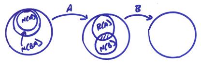
From I) we know that R(L) ![]() N(L*) = {0}. Thus, N(L) = N(L*L).
N(L*) = {0}. Thus, N(L) = N(L*L).
Solutions of linear mappings Lv
= w
1) Lv = w where L is one to one.
The matrix A representing L is square, DetA ![]() 0. The mapping is invertible and a unique
solution occurs. For this case, N(L) =
{0} and Rperp(L) = {0},
0. The mapping is invertible and a unique
solution occurs. For this case, N(L) =
{0} and Rperp(L) = {0},
2) Lv = w where L is not one to one.
For this case, N(L) ![]() {0}, but Rperp(L)
= {0}, a compatible system. There will
be a nonunique solution and we want to find the minimum norm solution, which is unique.
{0}, but Rperp(L)
= {0}, a compatible system. There will
be a nonunique solution and we want to find the minimum norm solution, which is unique.
3) Lv
![]() w. This is an
incompatible solution, and we want to find the best approximation to w in R(L). This may result in an unique or nonunique
solution v. For the nonunique case, find the minimum norm
solution.
w. This is an
incompatible solution, and we want to find the best approximation to w in R(L). This may result in an unique or nonunique
solution v. For the nonunique case, find the minimum norm
solution.
Case 1) – Lv = w and L is invertible. L is 1 to 1, (N(L) = {0}, and Rperp(L) = {0} (the system is compatible).
Ex)
L = A:RN ![]() RM where M=N, then
RM where M=N, then
Ax = y, and x = A-1y
where
A-1A = AA-1 = I
and
![]()
where the Adjugate(A) is the transpose of the cofactor matrix.
Ex)
![]()
Since DetA = -1 ![]() 0, the matrix A is an invertible square matrix,
and
0, the matrix A is an invertible square matrix,
and
![]()

Case 2) – Lv = w where
v is not unique. For this case, N{L} ![]() {0}, and we want to
find the minimum norm solution.
{0}, and we want to
find the minimum norm solution.
We can
write V as V = N(L) +Nperp(L) or v
= v1 + v2 where v2 is the unique part
of the solution. Show this by picking ![]() , then
, then
![]()
which implies v2
= ![]() . Since N(L) is perpendicular
to Nperp(L), then || v
||2 = || v1
||2 + || v2
||2. The minimum norm
solution consists of picking || v1
|| = 0. Thus, || v ||2 = || v2
||2.
. Since N(L) is perpendicular
to Nperp(L), then || v
||2 = || v1
||2 + || v2
||2. The minimum norm
solution consists of picking || v1
|| = 0. Thus, || v ||2 = || v2
||2.
2a) Let L be
represented by A:RN ![]() RM where N(A)
RM where N(A)
![]() {0}, N > M.
{0}, N > M.
We want a solution v2 in Nperp(A).
Since we have assumed no data errors, this is a purely underdetermined problem. Since Rperp(A) = {0}, then Dim R(A) = M and R(A) = W. Since Dim Nperp(A) = Dim R(A), then Dim Nperp(A) = M Dim N(A) = N-M.
In the case of a continuous Earth, N can be large and we may want to work in the smaller dimensional RM space. This might include the case where V is a signal space.
The solution v of Lv = w can be decomposed into

We want the part of solution v2 in Nperp(L). This is the minimum norm solution.
Now for any ![]() , then
, then ![]() where v2
where v2 ![]() R(L*) and thus v2
R(L*) and thus v2 ![]() Nperp(L),
since R(L*) = Nperp(L) from Adjoint Theorem I. Then,
Nperp(L),
since R(L*) = Nperp(L) from Adjoint Theorem I. Then, ![]() and
and ![]() forms a compatible
system (assuming
forms a compatible
system (assuming ![]() ). This will always be
the case for the purely underdetermined case.
). This will always be
the case for the purely underdetermined case.
Thus, if Rperp(L) = {0} = N(L*), the operator LL* is invertible and, from the Adjoint Theorem III, N(LL*) = N(L*) = {0}. Thus, LL* can be represented by an invertible M x M matrix (assuming W = RM) and
v2 = L*(LL*)-1w
is the minimum norm solution for the purely undertermined case.
If Rperp(L)
![]() {0}
{0} ![]() N(L*) = N(LL*), then
LL* is not invertible, but we can
still follow the prescription
N(L*) = N(LL*), then
LL* is not invertible, but we can
still follow the prescription
![]() (1)
(1)
![]() (2)
(2)
for any ![]()

If we can
find any solution to (1) for ![]() , then pushing it back through L* will give v2.
, then pushing it back through L* will give v2.
Ex) For a square matrix with N(L*) ![]() 0, then Rperp(L)
= N(L*) = N(LL*)
0, then Rperp(L)
= N(L*) = N(LL*) ![]() 0. Thus, LL* is not invertible even for some
square matrix cases.
0. Thus, LL* is not invertible even for some
square matrix cases.
Case 3) – Lv
![]() w
w
Ex)  . In this case, there
cannot be a x that gives an unequal b1 and b2.
. In this case, there
cannot be a x that gives an unequal b1 and b2.

In this
case, we want the best approximation
to w in R(L). Thus, we want to minimize || w
- Lv ||2 = || e ||2. Once we have found w1 ![]() R(L) where || w – w1 ||2 is minimized, we can either
have
R(L) where || w – w1 ||2 is minimized, we can either
have
a) solution v is unique and N(L) = {0}
b) solution v
is non-unique. For this case, find the minimum
norm solution ![]()
First, decompose w,
Lv ~ w = w1 + w2
where

Define w1
![]() R(L) such that Lv = w1. Then,
Lv ~ w = w1
+ e where e = w2. We want
e perpendicular to R(L). Then,
R(L) such that Lv = w1. Then,
Lv ~ w = w1
+ e where e = w2. We want
e perpendicular to R(L). Then,
L*Lv ~ L*w = L*(w1) + L*(e)
If e ![]() Rperp(L) =
N(L*), then L*(e) = 0 and L*Lv = L*w. If e = w2, then from the projection theorem, e has the minimum length. This forms a consistent set of equations
called the “normal equations” with e
= w2
Rperp(L) =
N(L*), then L*(e) = 0 and L*Lv = L*w. If e = w2, then from the projection theorem, e has the minimum length. This forms a consistent set of equations
called the “normal equations” with e
= w2 ![]() Rperp(L).
Rperp(L).
3a) Let N(L) = {0} = N(L*L). This is the purely overdetermined case for M > N.
L*L is then invertible and v = (L*L)-1 L*w. This is the best approximation solution.
Ex) Ax
= b where 
This type of system arises in multiple observations of a given parameter. First determine the four fundamental subspaces.
R(A) is spanned by the columns of
A. A basis is![]() .
.
Rperp(A) is then spanned
by ![]() .
.
Nperp (A) is spanned by the rows of A. The basis is (1).
N(A) = {0}.
Since N(A) = {0}, we need not worry about nonuniqueness, only incompatibility.
Any vector b ![]() Rperp(A)
cannot be reached by the operator A.
Thus,
Rperp(A)
cannot be reached by the operator A.
Thus,
![]() where bII
where bII ![]() Rperp(A)
Rperp(A)
Any vector with a nonzero bII has a component of b ![]() Rperp(A). Thus in general, this will form an
incompatible system
Rperp(A). Thus in general, this will form an
incompatible system

Typically, values of b
![]() Rperp(A)
are caused by
Rperp(A)
are caused by
1) a poorly formulated model problem
2) measurement errors in b which can’t be predicted by the model
This problem was first formulated by Gauss and Legendre and is known as the method of least squares method for obtaining a compatible system. It is a primary method today for making theory and data compatible.
To find the
best approximation to Ax ![]() b, form the normal equations
A*Ax = A*b. For the example above
b, form the normal equations
A*Ax = A*b. For the example above
A*A = 2 (A*A)-1 = ![]() , A*b
= [b1 + b2]
, A*b
= [b1 + b2]
xB.A. = (A*A)-1A*b = ![]() [b1 + b2]
[b1 + b2]
Thus, the inverse solution is simply the average of the observations.
Also, bI
![]() R(A) is then
R(A) is then

and

3b) Lu ![]() w and N(L)
w and N(L) ![]() {0}
{0}
Now we have both an incompatible system and a nonunique solution. This case is best handled with the singular value decomposition or SVD, but we attempt here to use adjoints.
First, kill off the part of w in Rperp(L) by forming the normal equations
L*Lv = L*w
Write this as
![]() with
with ![]()
Since N(L) ![]() {0}
{0} ![]() N(L*L)
N(L*L) ![]() N(
N(![]() ), this system is nonunique and
), this system is nonunique and ![]() = L*L is not
invertible. We need to find the minimum
norm solution. Chose any
= L*L is not
invertible. We need to find the minimum
norm solution. Chose any ![]() , then
, then
![]()
where
![]()
and
![]()
But since ![]() , then
, then
![]()
and the equation is not invertible.
Find any solution to ![]() . Then push
. Then push ![]() back through
back through ![]() to find the minimum
norm solution
to find the minimum
norm solution
![]()
This procedure is sometimes called the generalized inverse resulting in the minimum norm – best approximation solution.
Finally, other information may be
used to find the components v1
![]() N(L) in the solution
for v. Thus,
N(L) in the solution
for v. Thus,
![]()
where P is the dimension of the nullspace N(L). The ![]() can then be chosen to
satisfy the additional constraints on the problem.
can then be chosen to
satisfy the additional constraints on the problem.
Finally, one can modify orthogonality by changing the inner product. Hence, the adjoint operators and the inverse operators can be changed by changing the inner product! Thus, optimality is, in some sense, in the eye of the beholder.
In a following section, we will derive some solutions for the generalized inverse operators by developing spectral and generalized spectral methods in terms of the singular value decomposition or SVD. This will provide closed form solutions for the incompatible and nonunique case 3b).