EAS 657
Geophysical Inverse Theory
Robert L. Nowack
Lecture 9
Statistical Aspects of Inverse Theory
The generalized inverse gives the best approximation-minimum norm solution in the least squares sense. This is a valid procedure if the data are equally good, but this is generally not the case and some data are more prone to errors than other data. In addition, sometimes the data may be correlated. Also, the generalized inverse minimizes the length of the solution vector, so we should typically solve the problem

where x0 is some more reasonable starting solution than x = 0. However, note that this is not identical to Ax = y since x0 may have a nullspace component.
When we have some knowledge concerning the data noise and the probability of the model values, we can use this information to give more statistically significant results. (We will also be using this information to modify our inner products).
If the statistics are Gaussian, the resulting solution, given the data noise and the model probabilities, is known as the stochastic inverse.
The best known and easiest statistical distribution to use is the Gaussian or normal distribution. Fortunately, because of central limit theorem, sums of variables tend to Gaussian distributions regardless of the distribution of errors of the individual variables! (technically this is for i.i.d. variables; where the first “i” means independent, the second “i” and “d” means identically distributed).
The Gaussian distribution is a probability density function of the form

where N means normal, m
is the mean and ![]() is the variance.
is the variance.
i.e.  and has a zero mean
and unit variance. The general Gaussian
PDF is shown below
and has a zero mean
and unit variance. The general Gaussian
PDF is shown below
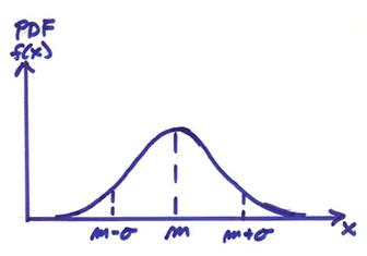
where
m ![]() includes 68% of the area under the probability density
function
includes 68% of the area under the probability density
function
![]() includes 95%
includes 95%
![]() includes 99%
includes 99%
This is sometimes called the (68, 95, 99) rule for the Gaussian pdf.
We will now introduce the moment
generating function (mgf) (an integral transform similar to a

This can be used to generate the moments of f(x). For the Gaussian pdf, this can be found directly to be
 (1)
(1)
Now,

where 1 is the total probability.

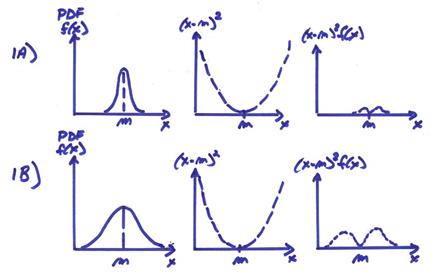
where this is the first moment of f(x) and m is the average value of the “random variable x from Eqn. (1). Next,

where this is the second moment of f(x) from Eqn. (1). Note that
![]()
Recall that ![]() is the variance. Thus,
is the variance. Thus,

PDF functions with small and large variances are shown below.
Claim: Convolution of pdf’s in the x-space is the product of the mgf’s in
the ![]() -space.
-space.
Much of statistics is based on this Fourier type of transform identity.
We now want to consider two variables, x1 and x2, each with errors which are normally distributed. Thus
x1 has a pdf ![]()
x2 has a pdf ![]()
We will assume that f1(x1) doesn’t depend on x2 and vice versa, i.e., the variables are statistically independent. What is the pdf of the variable y = x1 + x2?
Now, from basic probability, the “joint pdf” for more than one variable, which are statistically independent, is given by the product of the single variable pdf’s. (This can be used as a definition of statistical independence of random variables x1, x2). Thus,
![]()
Now consider the pdf of variable y (where y = x1 + x2) in a small region of f(x1,x2) = f1(x1) f2(x2)
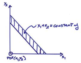
then
![]()
and
![]()
Now
letting ![]() , this can be written as
, this can be written as

This
is a convolution integral and from this fact we know that the mgf’s multiply,
thus ![]() (This is a Fourier
identity, that for the convolution of the two pdf’s, the mfg’s multiply). Then,
(This is a Fourier
identity, that for the convolution of the two pdf’s, the mfg’s multiply). Then,

This is also a Gaussian mgf with the form

where
![]() the means add for y = x1
+ x2
the means add for y = x1
+ x2
![]()
![]() the variances add for y = x1
+ x2
the variances add for y = x1
+ x2
Thus, both means and variances add,
and ![]() .
.
Now assume N Gaussian variables and y = x1 + x2 + … + xN, then
![]()
![]()
Therefore,

for the case where each xi has independent and identical Gaussian pdf’s.
Now if y = ax, then <y> = a<x> and <y2> = a2<x2>, then
![]() for y = ax
for y = ax
and

Ex) Let  , the average of N measurements xi, where the xi
are independent and identically, Gaussian distributed with
, the average of N measurements xi, where the xi
are independent and identically, Gaussian distributed with ![]() . Now, X is just the
computed average of these variables. What
is the pdf of X? Use the mgf function to
obtain this where
. Now, X is just the
computed average of these variables. What
is the pdf of X? Use the mgf function to
obtain this where

and

Thus, the average of a set of
measurements has the same mean as the individual xi, but with a reduced variance ![]() .
.
Thus, taking a number of estimates and averaging then reduces the variance of the sample mean where

has a mean m and standard deviation of the mean
![]()
Taking an average over N observations gives us a more reliable estimate of the mean m for the individual xi, provided the xi are i.i.d. Gaussian variables. If this were not the case, there would be no sense in repeating experiments.
Note, for some probability distributions, such as the Cauchy distribution, the standard deviation of the sample mean X is no smaller than the individual xi. Thus, there is no sense doing experiments more than once for random variables with this type of pdf.
Ex) Assume each seismogram can be represented by random variables x(ti)
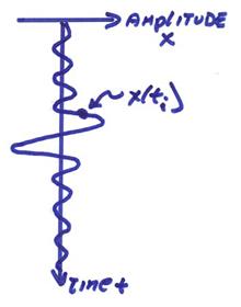
In a completely statistical sense, each discrete point of the seismogram can be viewed as a value of a random variable x(ti).
There has been a lot of work on measuring the ambient seismic noise level in the Earth which is found to result from random Rayleigh waves excited by wind, domestic noise, tides, etc. We will also use the term noise for any incoherent signals in the seismogram that we can’t model or that interfere with the signal we are interested in.
Ex) Assume we have
a repeatable, but weak seismic source and we want to enhance our signal to
noise. We will assume that the
background noise is Gaussian with a standard deviation about zero of ![]() . Repeat the
experiment N times and get N seismograms as shown below.
. Repeat the
experiment N times and get N seismograms as shown below.
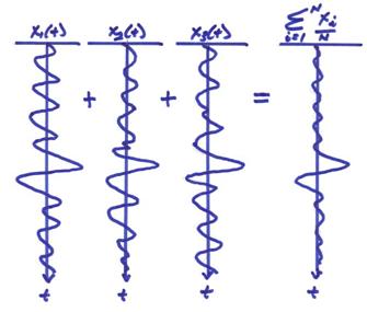
If the noise is i.i.d.
Gaussian, then simply by adding the repeated traces point by point and dividing
by N, we will reduce the noise level by ![]() with respect to the non-random
signal. This type of signal to noise
enhancement is called “stacking”.
with respect to the non-random
signal. This type of signal to noise
enhancement is called “stacking”.
Ex) Assume we have a seismic plane wave from distant source and a group of receivers in a seismic array.
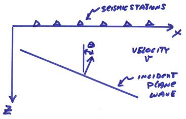
The recorded seismic arrivals
with time will arrive at each station at different times depending on the angle
![]() with respect to the
vertical of the incident plane wave.
with respect to the
vertical of the incident plane wave.
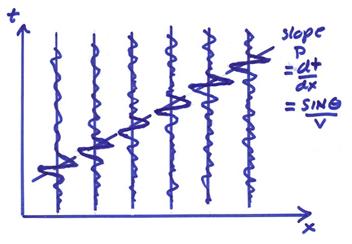
In order to enhance the signal arriving at the array at this slope p, then perform a delay in order to align the arrival of interest followed by a stacking operation. Thus,
![]()
or writing this as an integral of position as
![]()
This is a shift and stack operation.
In earthquake seismology, this type of operation is called “seismic beamforming”. In exploration seismology, this is called a “slant stack”. In either case, the “coherent signal” arriving at the slope p across the array will be enhanced with respect to the incoherent signals.
If the incoherent parts of the signal are i.i.d.
Gaussian, then the coherent signal will be enhanced with respect to the noise
by ![]() , where N is the number of traces stacked.
, where N is the number of traces stacked.
Ex) A CMP (common midpoint) stack. There are many new ideas in this procedure and we will discuss them one at a time.
Seismic reflection data is recorded in common shot gathers. If enough common shot data is recorded, the data can be reorganized into common midpoint gathers as shown below.
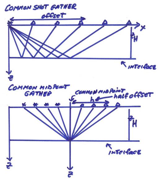
a) The first important idea is to rearrange the seismic data (assuming we have multiple sources and receivers) into midpoint and half offset coordinates with
![]() = source locations
= source locations
![]() = receiver locations
= receiver locations
Thus,

For a single common midpoint Xm, this would result in a CMP seismic gather. The utility of this coordinate change is that now all data in a CMP gather scatter near the same point in the subsurface. This data reorganization is mostly done in seismic exploration, but earthquake seismologists could also benefit from this modified coordinate frame. Thus, for each midpoint, we have a number of half-offsets.
b) For a homogeneous layer and one interface in the subsurface, we can calculate the travel time as

where v is the speed in the layer and ZH is the layer thickness. This equation is a circle in (ZH,h) space and a hyperbola in (h,t) space. The data in (h,t) is shown below.
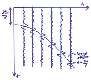
Now, we want to plot at each midpoint coordinate a representative trace corresponding to the reflectance of the subsurface interface at that point. We could just plot the near offset trace, but this in general will be quite noisy due to source induced surface waves (ground roll) and other noise at the surface. We will shift in time every trace by a hyperbolic “normal moveout” time and stack to reduce noise. Then, plot this stacked trace at the midpoint.
But, we have to make several adjustments, including adjusting each trace for local topography and weathering zones. These are called static time corrections to make the arrivals better fit a hyperbolic moveout. For a vertically varying medium, we can still use the hyperbola formula for small offsets, but we need to replace a constant v by an RMS velocity down to the reflector. Also, we would need to stretch the individual traces as well.
Finally, after the normal moveout, we would stack the traces as
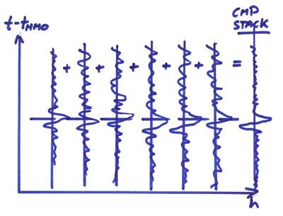
![]() a CMP Stack
a CMP Stack
This is one of the most important procedures in reflection seismology. It results in a greatly increased signal to noise for the stacked trace. But, if there is significant laterally velocity variations (or if the statics are wrong) then the coherent signals will not stack properly giving a sub-optimal stacked result.
This procedure can also be used to perform velocity analysis since the shape of the hyperbolic moveout is dependent on the velocity v.
Multi-Dimensional
Gaussian Random Variables
For independent Gaussian variables, then the joint pdf is
![]()

We want to generalize this Gaussian form for non-independent
correlated variables. Let ![]() , where x is
a vector of random variables. Then,
, where x is
a vector of random variables. Then,

where Bij is a symmetric matrix. Or,
![]()
For this to be valid pdf, then
![]()
This can be used to find the normalizing factor giving

For ![]() not to blowup, then B
must be a “positive definite” NxN matrix (i.e., all its singular values must be
positive).
not to blowup, then B
must be a “positive definite” NxN matrix (i.e., all its singular values must be
positive).
What is the interpretation of B? It turns out that
![]()
and is the covariance matrix for x, where
![]()
and
![]()
The general multivariable Gaussian pdf is then,

Assuming the model and data vectors are random Gaussian variables, then the pdf for the data is

The relation between <y> and some model parameters x can be given by a relation g(x) = y. For a linearized forward model then, Ax = y and our object is to find the xi, i = 1,N, that maximizes the pdf f(y1,y2,…,yM) given Ax = y. Thus,

For the Gaussian pdf, this can be done by finding x such that the exponent is minimized. In statistics, this is called the maximum likelihood method – a workhorse of statistics. We can maximize the pdf by minimizing,
![]() (1)
(1)
If the initial model probabilities give us a prior model x0 and covariance ![]() , we might want to also simultaneously minimize:
, we might want to also simultaneously minimize:
![]() (2)
(2)
Note that the damped least squares inverse minimizes both eqns. (1) and (2) with

Bayes Theorem
The minimizations above can be
viewed in terms of Bayes Theorem.
Consider the joint pdf f(x1,x2) where ![]() . An example of a
joint pdf is shown below.
. An example of a
joint pdf is shown below.
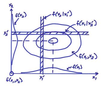
The individual pdf’s can be obtained from the joint pdf f(x1,x2) as
![]()
This is called “marginalization” and removes other
parameters by integration of the joint pdf.
Extraneous variables are sometimes called “nuisance” parameters which
can be removed by marginalization. From
the above figure, the probability conditioned on ![]() can be written
can be written
![]()
Similarly,
![]()
Letting ![]() and
and ![]() be arbitrary then,
be arbitrary then,
![]()
or
![]()
This is called Bayes Theorem. If we assume that x2 is a model parameter and x1 is a data parameter, then Bayes theorem can be written as
![]()
where f(data|model) is called the likelihood function for the forward model, f(model) is the pdf for the prior model with no influence from the data, and f(data) is called the evidence and can be viewed as a normalization factor. Thus,
f(model|data) ~ f(data|model) f(model)
If y corresponds to the data, x to the model parameters, and the relation between the model and data is y = Ax, then the pdf of the data given the model can be written as
f(data|model) ~ ![]()
and the pdf for the prior model can be written as
f(model) ~ ![]()
Thus, from Bayes Theorem we would like to maximize the conditional pdf of the model given the data
f(model|data) ~ ![]()
or minimize the exponent
![]()
If ![]() and
and ![]() , then minimizing this will result in the damped least
squares solution as we will see in the next lecture.
, then minimizing this will result in the damped least
squares solution as we will see in the next lecture.