

Interpreting Seismograms - A Tutorial
for the AS-1 Seismograph 1
|
|
Larry BraileProfessor,
http://web.ics.purdue.edu/~braile/ October, 2006, updated January, 2007 |

Objective: This tutorial is intended as a resource for the interpretation of seismograms recorded by educational seismographs. The tutorial provides a description of the main features of the Earth that affect seismic wave propagation and therefore controls the character of seismic signals recorded on seismographs. A catalog of selected seismograms is also presented to illustrate the variation in signal properties with distance, magnitude, and depth of focus. After initial visual analysis of an earthquake seismogram, one can often determine additional information about the event by identifying phases (individual arrivals on the seismogram that travel a distinct path through the Earth) and measuring amplitudes to estimate the magnitude of the earthquake.
This tutorial is available for viewing with a browser (html file) and for downloading as an MS Word document or PDF file at the following locations:
http://web.ics.purdue.edu/~braile/edumod/as1lessons/InterpSeis/InterpSeis.htm
http://web.ics.purdue.edu/~braile/edumod/as1lessons/InterpSeis/InterpSeis.doc
http://web.ics.purdue.edu/~braile/edumod/as1lessons/InterpSeis/InterpSeis.pdf
A PowerPoint presentation for the Interpreting
Seismograms document is available for download at: http://web.ics.purdue.edu/~braile/edumod/as1lessons/InterpSeis/InterpSeis.ppt
Contents (click on topic to go directly
to that section; use the red up arrows to return to the list of contents):
1. Introduction
2. Seismic Wave Propagation in the Earth
3. Catalog of Seismograms
at Various Distances – Screen Images
4. Catalog of
Seismograms at Various Distances – 60-minute Seismograms
5. Catalog of
Seismograms for Different Magnitudes – Distance ~ 30o
6. Catalog of
Seismograms for Different Magnitudes – Distance ~ 60o
7. Catalog of
Seismograms for the Same Magnitude (~6.7) at Different Distances
8. Catalog of
Seismograms for Large Earthquakes at About the Same Distance
9. Catalog of
Seismograms for the Same Distance (~65o) for Different Depths of
Focus
10. Analysis of Noise on
Seismograph Records
11. Mystery Events
12. References
1. Introduction:
Interpreting
earthquake seismograms generally requires considerable experience and study of
seismology. However, there are some
fundamental principles that provide a basic understanding of seismic wave
propagation and seismogram characteristics.
Furthermore, some experience can be quickly obtained by systematic study
of selected seismograms illustrating variations in amplitude and signal
character related to source-to-station distance, the magnitude of the
earthquake, and the earthquake’s depth of focus.
This tutorial utilizes seismograms recorded over the last six years at
the WLIN station in
An earthquake
catalog (Excel file) for the WLIN station can be downloaded at: http://web.ics.purdue.edu/~braile/edumod/as1lessons/InterpSeis/EqList.xls. Sample AS-1 seismic data for the WLIN station
for the years 2004 and 2005 (data for days that have no significant events have
been deleted from the files to reduce the total file size; files are compressed
and are zip files; the 2004 file is 17.2MB; the 2005 file is 46.4MB; files must
be unzipped [extracted] and placed in your AmaSeis folder to view with the
AmaSeis software as folders named “2004” and “2005”) are available at: http://web.ics.purdue.edu/~braile/new/2004.zip
and http://web.ics.purdue.edu/~braile/new/2005.zip. You can use these data with the AmaSeis
software to view and analyze seismograms, determine the epicenter-to-station
distance using the S minus P method and calculate magnitudes.
![]()
Return to list of contents
2. Seismic Wave Propagation in the Earth: Four main types of seismic waves propagate in elastic materials including the Earth. A simplified model of Earth’s interior structure is illustrated in Figure 1. A hands-on Earth structure activity is available at: http://web.ics.purdue.edu/~braile/edumod/earthint/earthint.htm. Two types of body waves, compressional or P-waves and shear or S-waves, travel through the Earth’s interior. S-waves do not travel through fluids so they are not present in the Earth’s liquid outer core. The two types of surface waves are Rayleigh waves and Love waves. Surface waves travel approximately parallel to the Earth’s surface and their particle motions decrease in amplitude with depth below the surface. Additional information of seismic waves can be found in standard seismology and Earth science reference books including Bolt (1993, 2004) and Shearer (1999). Hands-on activities for exploring seismic waves and seismic wave propagation using the slinky are available at: http://web.ics.purdue.edu/~braile/edumod/slinky/slinky.htm and
http://web.ics.purdue.edu/~braile/edumod/slinky/slinky4.htm.
Seismic wave animations and related hands-on activities are be found at:
http://web.ics.purdue.edu/~braile/edumod/waves/WaveDemo.htm.
Seismic waves in the Earth can be represented by specific raypaths and
wave types that result in distinct arrivals, called phases, on seismograms
(Figure 2). Several raypaths for seismic
phases and the concept of geocentric angle (angular distance) and distance
along the Earth’s surface are illustrated in Figures 2, 3 and 4.
Travel times for seismic waves are well known from many years of recording seismograms all over the world from earthquake and explosive sources. Examples of standard travel time curves are shown in Figures 5, 6 and 7. These curves can be used to estimate the epicenter-to-station distance from the S minus P time (Figures 7 and 8) and for identifying phases (arrivals) on recorded seismograms. Examples of using the AmaSeis software and AS-1 seismograms for the S minus P distance estimation and epicenter location method are given at:
http://web.ics.purdue.edu/~braile/edumod/as1lessons/UsingAmaSeis/UsingAmaSeis.htm
http://web.ics.purdue.edu/~braile/edumod/eqdata/eqdata.htm
http://web.ics.purdue.edu/~braile/edumod/as1lessons/EQlocation/EQlocation.htm.
The magnitudes (mb, MS and mbLg) of earthquakes recorded on the AS-1 seismograph can also be estimated using methods described at:
http://web.ics.purdue.edu/~braile/edumod/as1lessons/EQlocation/EQlocation.htm
http://web.ics.purdue.edu/~braile/edumod/as1lessons/magnitude/CalcMagnElect.htm
http://web.ics.purdue.edu/~braile/edumod/as1mag/as1mag.htm
and the AS-1 online magnitude calculator:
http://web.ics.purdue.edu/~braile/edumod/MagCalc/MagCalc.htm. Magnitudes can also be calculated directly with the AmaSeis software.
Results of many magnitude calculations for WLIN seismograms are illustrated at:
http://web.ics.purdue.edu/~braile/edumod/MagCalc/AS1Results.htm.
Additional raypath diagrams for seismic wave propagation through the Earth are shown in Figures 9-12.
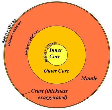
Figure 1.
Schematic diagram illustrating the major spherical shells of the Earth's
interior structure. The circles
(representing spherical shells in the 3-D model) are drawn at true scale except
for the circle representing the base of the crust. The thickness of the crustal layer is
exaggerated so that a distinct layer is visible at this scale (the scale of this
diagram is approximately 1:120 million).
In the real Earth, the crust is also of variable thickness with
significant differences between the crustal thickness of oceanic and
continental regions and increased crustal thickness beneath mountainous areas.
Figure 2. Segment of Earth model
showing main boundaries and layers, and approximate compressional- or P-wave
velocity with depth. Raypath shows
approximate travel path for the first arriving P-wave (and the S-wave) for the
seismogram shown above. The seismogram
was recorded by the
Figure 3. Cross
section through the Earth showing important layers and representative raypaths
of seismic body waves. Direct P and S raypaths (phases), including a
reflection (PP and pP), converted phase (PS), and a phase that travels through
both the mantle and the core (PKP). P raypaths are shown by heavy
lines. S raypaths are indicated by light lines. Additional
information about raypaths for seismic waves in the whole Earth and
illustrations of representative raypaths are available in Bolt (1993, p.
128-142) and Shearer (1999, p. 49-60). Surface wave propagation (Rayleigh
waves and Love waves) is schematically represented by the heavy wiggly
line. Surface waves propagate away from the epicenter, primarily near the
surface and the amplitudes of surface wave particle motion decrease with depth.
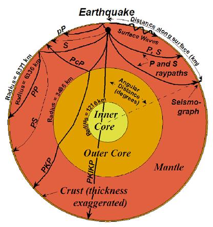
Figure 4. Earth structure and
raypaths (Figure 3) with the addition of a raypath for the seismic phase PKIKP
that travels through the Earth’s inner core.
Figure 5. Standard Earth travel
time curves for a source depth of 0 km (can be used for shallow focus earthquakes
at distances of ~20 to 120 degrees).
Travel times for many different phases (types of seismic waves and paths
through the Earth) are shown. Note that
the difference between the S and the
P times increases smoothly with distance.
Therefore, a seismogram with a given S minus P time will only match the
travel time data at one specific distance.
This diagram is available at: http://neic.usgs.gov/neis/travel_times/ttgraph.html.
Figure 6. Standard travel time
curves for the Earth for several seismic phases. Travel times for some primary phases are
highlighted.
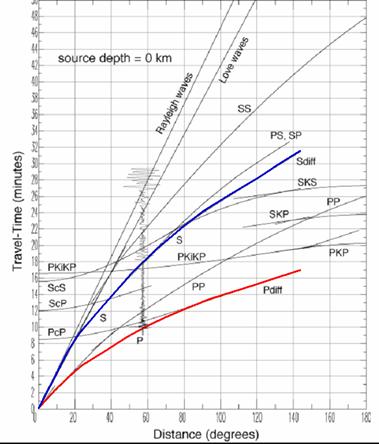
Figure 7. Overlaying a seismogram
(station KIP, M7.5, 1999
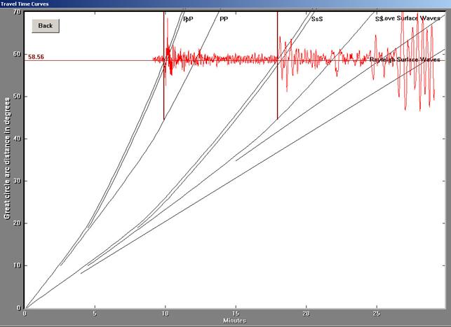
Figure 8. KIP seismogram for the
Figure 9. Raypaths and wavefronts for selected primary
(compressional) wave phases which travel through the Earth. The travel times (in minutes) along the
raypaths and the corresponding wavefronts (short dashed lines; lines or surfaces
of equal travel time) are given by the small numbers adjacent to the
wavefronts. The raypaths are
perpendicular to the wavefronts and represent the direction that a specific
point on the wavefront is propagating.
The raypaths in this real Earth model are curved because the seismic wave
velocity varies with depth. Note the
strong refraction (bending) of the raypaths and wavefronts caused by the
velocity change across the core-mantle boundary. The primary wave types (phases) illustrated
in this diagram are:
P Raypaths
for waves which travel through the mantle with a relatively direct path; 0°-103° distance
range.
Pdiffracted Raypaths for
waves which travel through the mantle and are diffracted at the core-mantle
boundary by the reduced outer core velocity; 103°-150° distance range.
PKP Raypaths for
waves which travel through the mantle, are strongly refracted at the
core-mantle boundary and travel through the outer core; 110°-187° distance
range.
PKIKP Raypaths for
waves which travel through the mantle, the outer core and the inner core; 110°-180° distance
range.
PKiKP Raypaths for
waves that are reflected from the inner core.
In more recent models of the Earth's interior, the PKiKP arrivals are
observed for distances less than about 120°.
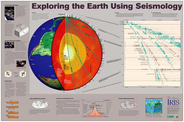
Figure
10. IRIS “Exploring the Earth Using
Seismology” poster illustrating seismic wave propagation through the Earth (http://www.iris.edu/about/publications.htm#p).
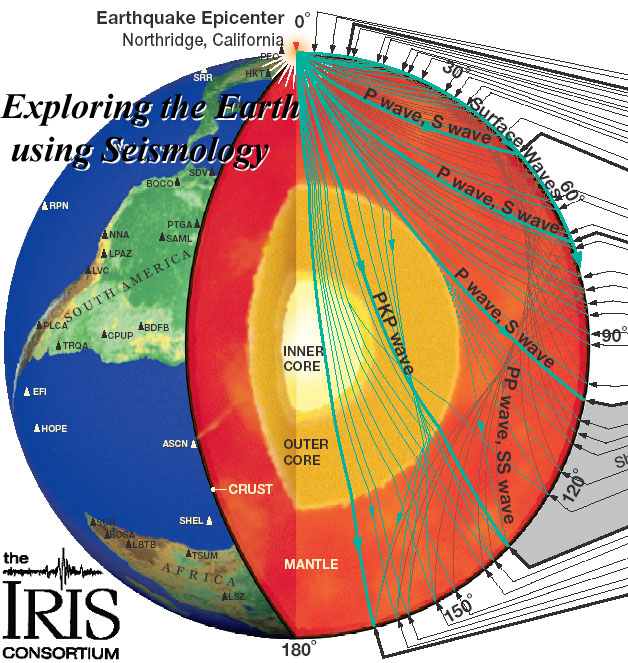
Figure 11. Close-up diagram of a
portion of the IRIS poster (Figure 10) showing raypaths through the Earth’s
interior for several seismic phases.
Distances in geocentric angle are noted using the degrees scale.
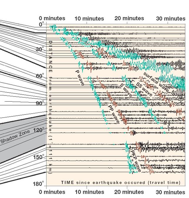
Figure 12. Close-up diagram of a
portion of the IRIS poster (Figure 10) showing a seismogram record section with
several phases identified.
![]()
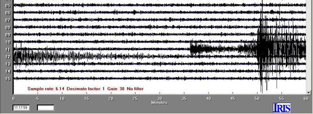
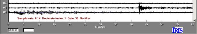
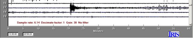
3. Catalog of Seismograms at Various Distances – Screen Images: The partial screen images (from the 24-hour display in AmaSeis for station WLIN) included below and labeled A through R show seismograms from shallow focus earthquakes at epicenter-to-station distances from 1.81 degrees to 143.49 degrees. All screen displays have the same gain factor of 30. The selected seismograms illustrate the change in character of seismic signals with increasing source-to-station distance. It is immediately clear that as the distance increases, the seismograms have longer time duration. This feature is caused be the fact that different wave types travel at different velocities which causes the difference in time between phases to increase with distance. An example is the S minus P times as illustrated in Figures 6 and 7. Also, surface waves travel slower than S waves and are dispersive (velocity is a function of frequency) further increasing the duration of the seismogram with increasing distance of travel. Furthermore, greater source-to-station distance tends to result in many phases representing different wave types and travel paths to have similar amplitudes so that the seismograms are often long and complex. Seismograms also often show a relatively abrupt first arrival (P wave energy), a small number of distinct arrivals, and then a slow “tapering off” of amplitudes as time increases. This last part of the seismogram is called the “coda.” Some of the records shown below also include signals from other events and several noise sources.
Additional information about the events represented by the seismograms can be found in the Excel spreadsheet station catalog (http://web.ics.purdue.edu/~braile/edumod/as1lessons/InterpSeis/EqList.xls).
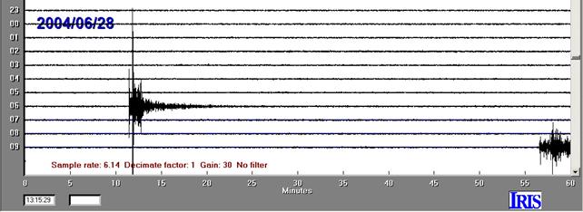
A.
D = 1.81o, 2004 6/28,
B.
D = 2.59o, 2002 6/18, Near
C.
D = 5.31o, 5/1/05,
D.
D = 9.30o, 2002 11/3,
E.
D = 14.68o, 2004 8/1, N.
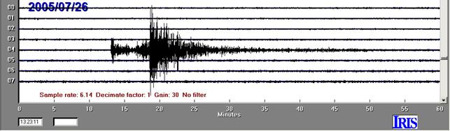
F.
D = 19.39o, 2005 7/26,
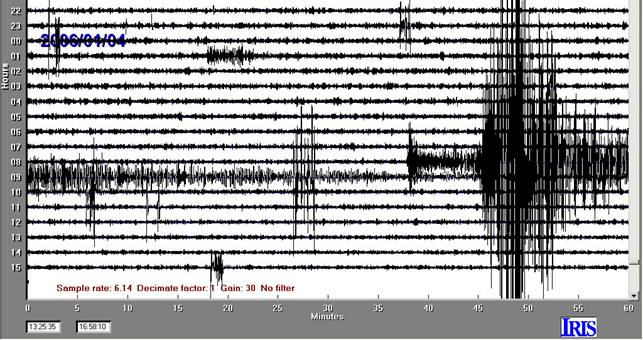
G.
D = 24.10o, 2006 1/4,
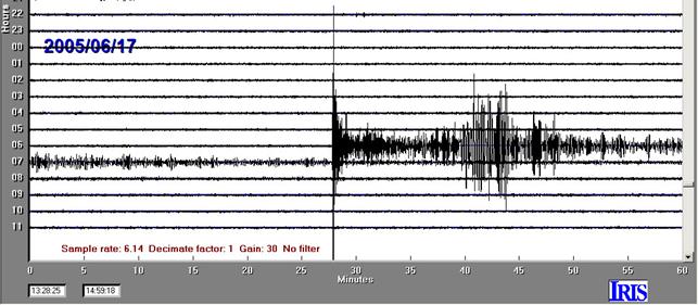
H.
D = 29.97o, 2005 6/17, Off
I. D = 42.04o, 2002 10/23,
J.
D = 51.92o, 2003 2/19, Unimak
Island Region,
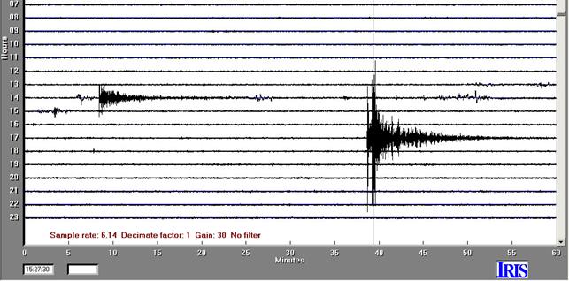
K.
D = 61.17o, 2005 6/14, Rat
Islands, Aleutians,
L.
D = 67.70o, 2003 5/21,
M.
D = 81.08o, 2000 8/4,
Sakhalin,
N.
D = 96.20o, 2004 9/5, Near
O.
D = 103.21o, 2005 10/8,
P.
D = 112.99o, 2001 1/26,
Q. D = 127.24o, 2003 8/21, S.
Island,
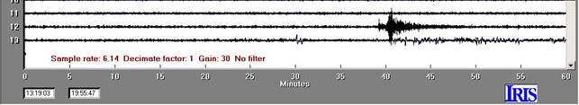
R.
D = 143.49o, 2000 6/4,
![]()
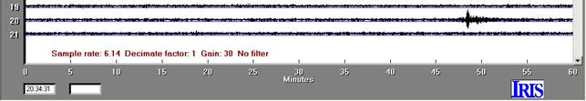
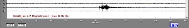
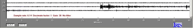
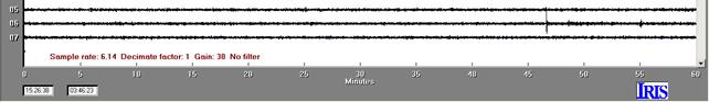
4. Catalog of
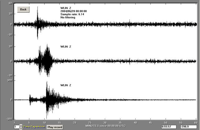
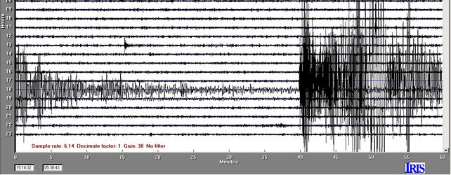
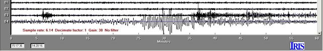
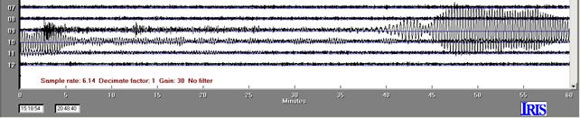
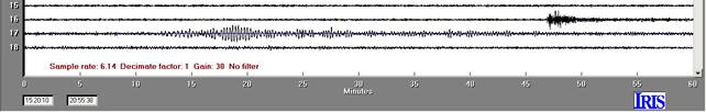
Seismograms at Various Distances – 60-minute Seismograms: In the following 3-trace plots (extracted using AmaSeis), the A through R seismograms shown above are displayed as 60-minute records (with
different amplitude scales – note the vertical scales on the left) to see a
direct comparison of the signals at various distances and the same time
scale. For some of the seismograms, one
could “zoom in” further using the AmaSeis extract seismogram tool to see more
detail. The digital, SAC-format
seismograms are listed (with Internet links) in Table 1 so that one can change
the view by “zooming in” and perform additional analysis and display the
results. Seismograms P, Q
and R are also shown in 2-hour
records because of the duration of these records due to the large
source-to-station distances. The
increase in duration with distance, characteristic phases and seismogram
complexity are apparent from the comparison of these seismograms.
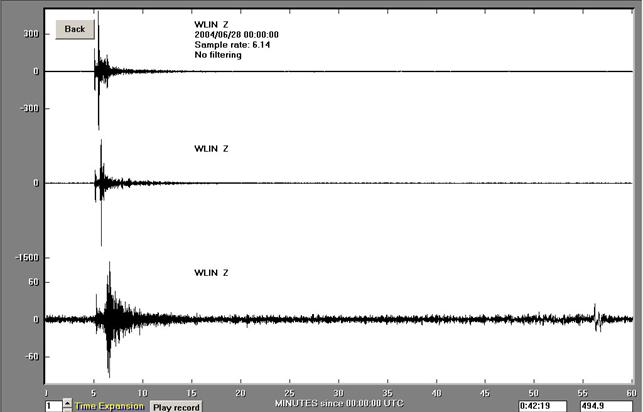
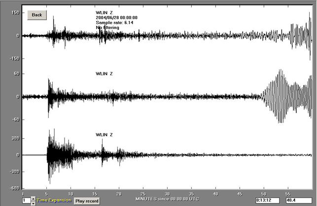
Seismograms A (D = 1.81o), B (D = 2.59o) and C (D = 5.31o).
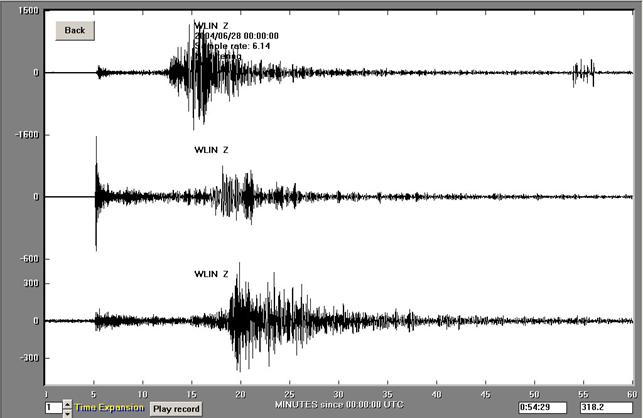
Seismograms D (D = 9.30o), E (D = 14.68o) and F (D = 19.39o).
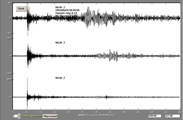
Seismograms G (D = 24.10o), H (D = 29.97o) and I (D = 42.04o).
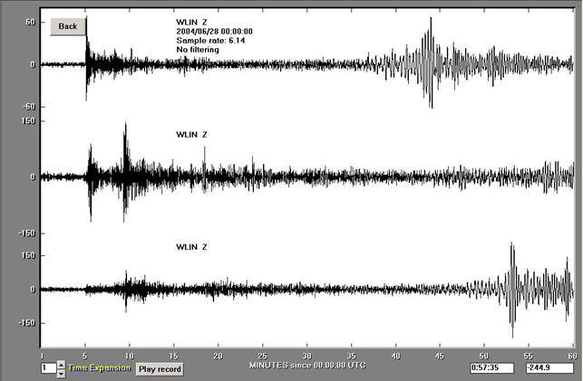
Seismograms J (D = 51.92o), K (D = 61.17o) and L (D = 67.70o).
Seismograms M (D = 81.08o), N (D = 96.20o) and O (D = 103.21o).
Seismograms P (D = 112.99o), Q (D = 127.24o) and R (D = 143.49o).
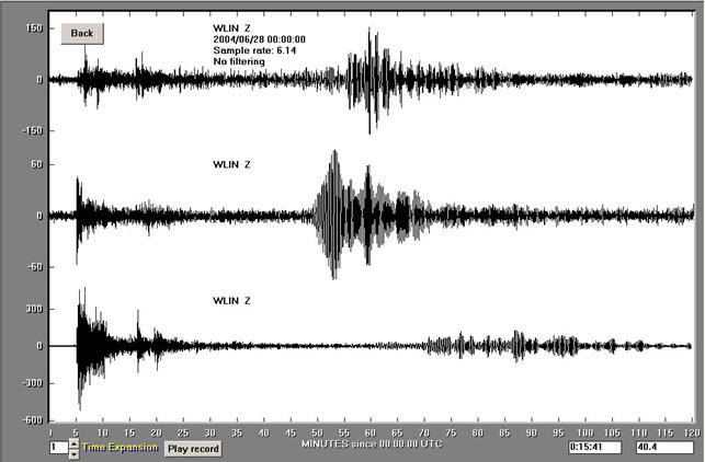
Seismograms P (D = 112.99o), Q (D = 127.24o) and R (D = 143.49o) (2- hour
seismograms).
Table 1. Seismogram download files for events at
various distances.
![]()
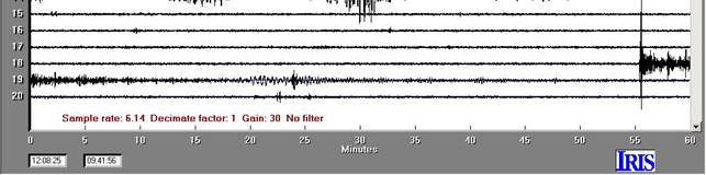
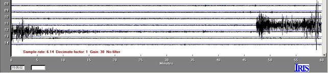
5. Catalog of Seismograms for Different Magnitudes – Distance ~30o: To illustrate the effects of different magnitudes of the earthquake on the seismogram, several seismograms from different magnitude events but with a source-to-station distance of about 30o are shown in 3-trace plots below (amplitude scale factor is the same for all traces). The seismograms are listed in Table 2 along with links to the digital files. It is clear that the general shape of each seismogram is similar (because of similar distances) but the amplitudes become significantly smaller with decreasing magnitude of the earthquake.
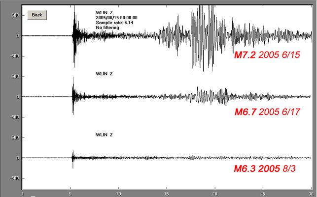
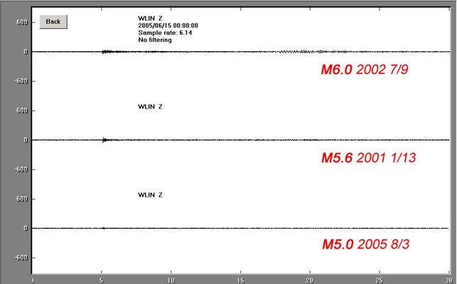
Table 2. Seismogram download files for magnitude
comparison for distance ~30o.
![]()
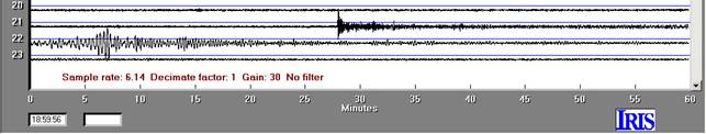
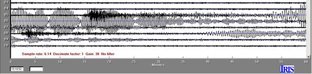
6. Catalog of Seismograms for Different Magnitudes – Distance ~60o: To illustrate the effects of different magnitudes of the earthquake on the seismogram, several seismograms from different magnitude events but with a source-to-station distance of about 60o are shown in 3-trace plots below (amplitude scale factor is the same for all traces). The seismograms are listed in Table 3 along with links to the digital files. It is clear that the general shape of each seismogram is similar (because of similar distances) but the amplitudes become significantly smaller with decreasing magnitude of the earthquake.
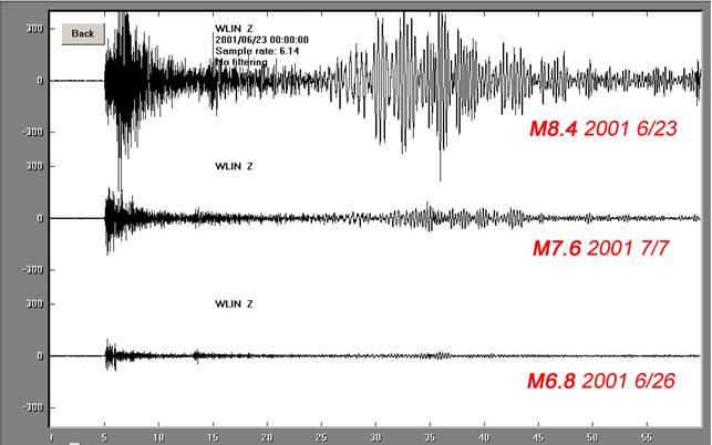
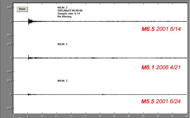
Table 3. Seismogram download files for magnitude comparison for distance ~60o.
![]()
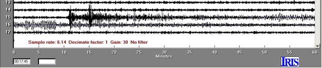
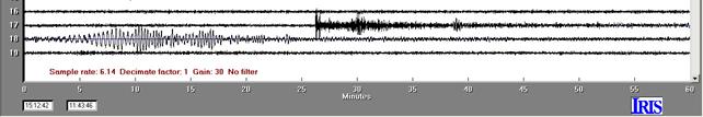
7. Catalog of Seismograms for the Same Magnitude (~6.7) at Different Distances: To illustrate the effects of magnitude and distance of the earthquake on the seismogram, several seismograms from the same magnitude events but with different source-to-station distances are shown in 3-trace plots below (amplitude scale factor is the same for all traces). The seismograms are listed in Table 4 along with links to the digital files. For the same magnitude earthquake the amplitudes of the seismograms become significantly smaller with increasing distance. One can also observe differences in the character of the seismograms with increasing distance similar to what was observed with seismograms A through R. The seismograms are listed in Table 4 along with links to the digital files.
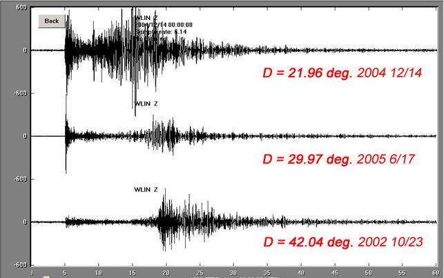
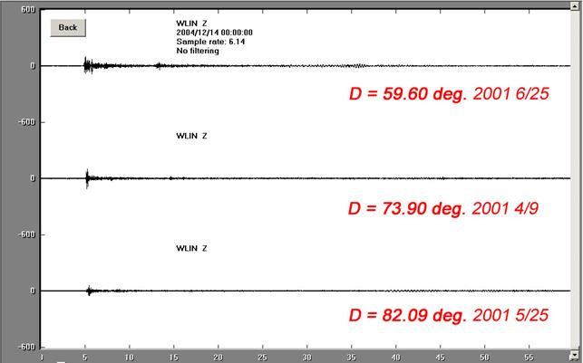
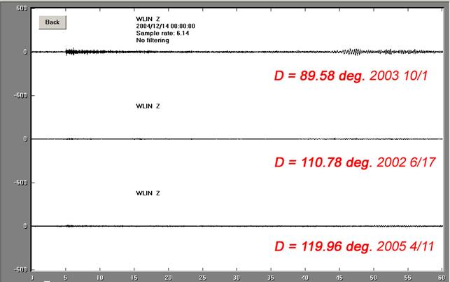
Table 4. Seismogram download files for magnitude comparison for various distances, M ~6.7.
![]()
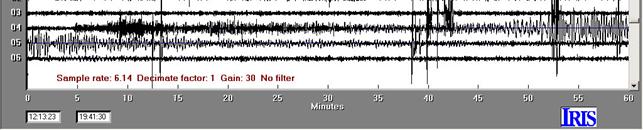
8. Catalog of Seismograms for Large Earthquakes at About the Same Distance: Seismograms for 3 large earthquakes from a source-to-station distance of about 130o are illustrated in the 3-trace plot below (amplitude scale factor is the same for all traces). The seismograms are listed in Table 5 along with links to the digital files.
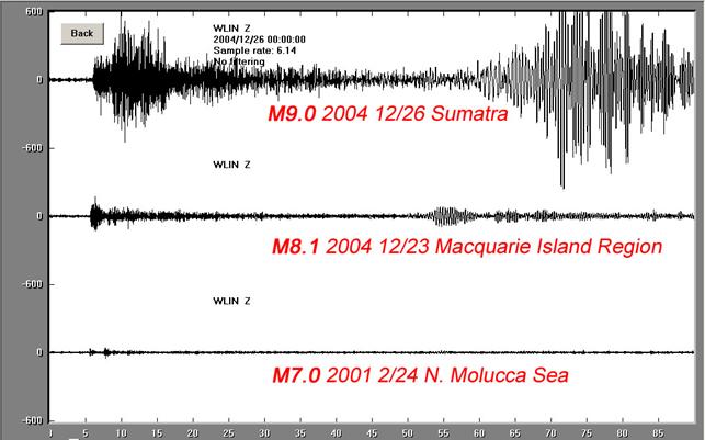
Table 5. Seismogram download files for magnitude comparison for distance ~130o.
|
Magn. |
Dist (Deg.) |
Seismogram |
|
M9.0 |
136.34 |
http://web.ics.purdue.edu/~braile/edumod/as1lessons/InterpSeis/0412260113WLIN.sac
|
|
M8.1 |
133.39 |
http://web.ics.purdue.edu/~braile/edumod/as1lessons/InterpSeis/0412231513WLIN.sac |
|
M7.0 |
128.45 |
http://web.ics.purdue.edu/~braile/edumod/as1lessons/InterpSeis/0102240749WLIN.sac |
Examination of many seismograms from various magnitude earthquakes recorded at different distances allows one to generalize the “detectibility” of events for the AS-1 seismograph. Figure 13 illustrates the approximate relationship between earthquake magnitude and maximum distance of detection (relatively clear seismogram visible on the record) for the WLIN AS-1 station.
Figure 13. Approximate maximum distance of recording for the AS-1 seismograph as a function of the magnitude of the source. Variation in the actual distance will occur due to noise levels, depth of focus of the earthquake, site response at the sensor and other factors.
![]()
9. Catalog of Seismograms for the Same Distance (~65o) for Different Depths of Focus: To illustrate the effects depth of focus of the earthquake on the seismogram, several seismograms from about the same source-to-station distance but different focal depth are shown in 3-trace plots below (amplitude scale factor is the same for all traces in the first set of seismograms but is different in the second set). The seismograms are listed in Table 6 along with links to the digital files. The major difference in the seismograms is the reduction of the surface waves for deeper earthquakes. Also, a prominent “depth phase” (pP) is visible on the seismograms just after the first P arrival. The pP minus P time can be used to accurately determine the depth of focus of the event.
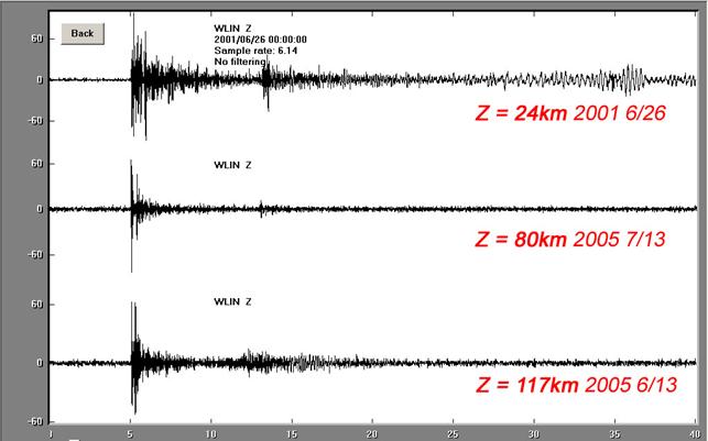
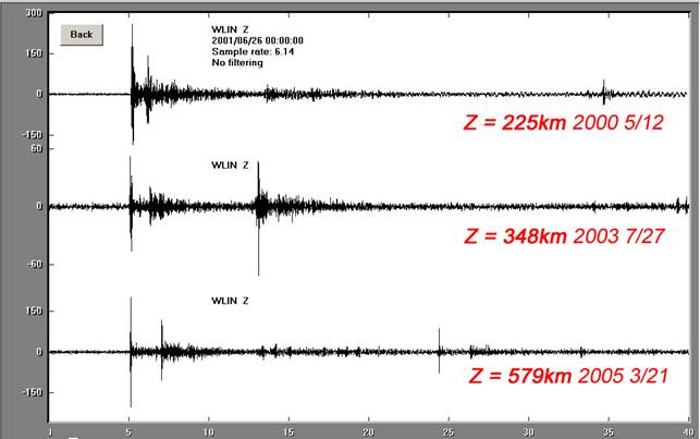
Table 6. Seismogram download files for depth of focus comparison for distance ~65o.
The P, pP and S phases for two of these earthquakes are illustrated on the seismograms shown in Figures 14 and 15 using the AmaSeis travel time curve display tool. The pP – P time (difference in arrival time of the pP phase and the P phase) can be used to accurately determine the depth of focus of the earthquake. Table 7 shows the pP – P times for various depths for an epicentral distance of 65 degrees.
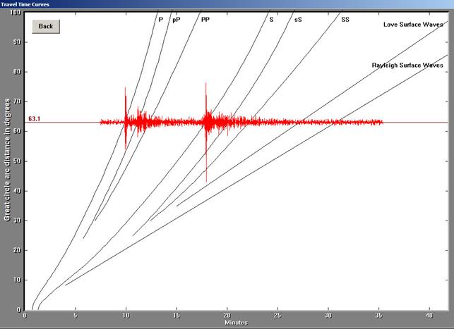
Figure 14. Seismogram for the
7/27/03 earthquake displayed using the AmaSeis travel time curve tool. A depth of 348 km was entered for this event
to produce the travel time curves. The
match of the pP – P time indicates that the depth of focus determined from this
seismogram is approximately correct.
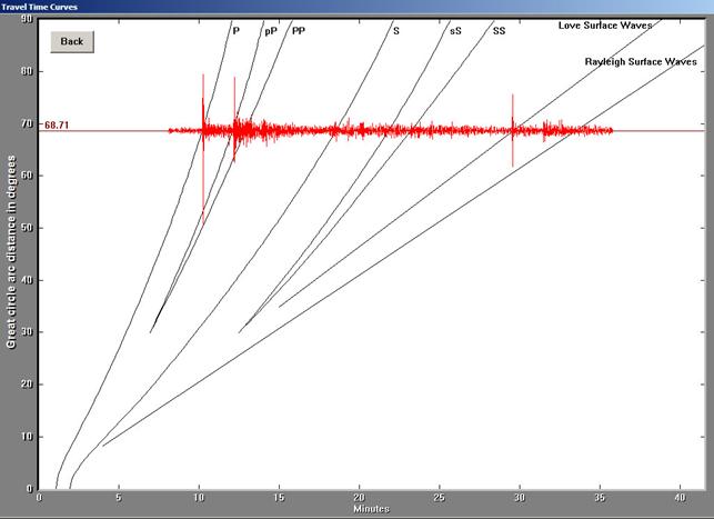
Figure 15. Seismogram for the
3/21/05 earthquake displayed using the AmaSeis travel time curve tool. A depth of 579 km was entered for this event
to produce the travel time curves. The
match of the pP – P time indicates that the depth of focus determined from this
seismogram is approximately correct.
Table 7. pP minus P times for the pP phase (depth
phase) for an epicenter-to-station distance of 65 degrees and various depths of
focus (hypocentral depths).
|
Depth |
pP - P Time |
|
(km) |
(seconds) |
|
0 |
0 |
|
50 |
14 |
|
100 |
25 |
|
200 |
46 |
|
300 |
67 |
|
400 |
86 |
|
500 |
102 |
|
600 |
118 |
|
700 |
133 |
![]()
10. Analysis of Noise on Seismograph Records: Signals are commonly visible on a seismograph
that are not caused by earthquakes or other seismic sources such as
explosions. These signals are often
referred to as “noise” and come from many possible sources. Noise on the seismograph record can
significantly affect the ability to detect or recognize an earthquake signal. Also, it is necessary to consider how one can
distinguish a seismogram signal from noise.
Some of the characteristics of earthquake seismograms have previously
been illustrated in the catalog sections above.
In this section, we will consider what factors affect the signals that
are visible on the seismograph and the characteristics of earthquake
seismograms and noise. A very
distinctive seismogram is illustrated on the AmaSeis partial screen display
shown in Figure 16. A list of factors
that affect the characteristics of the seismogram is given in Figure 17 and
schematically illustrated in Figure 18.
Figure 16. Example of a
distinctive seismogram characteristic of an earthquake generated signal. No large amplitude noise sources are visible.
Figure 17. List of factors that
affect the seismic signals that are visible on the seismograph.
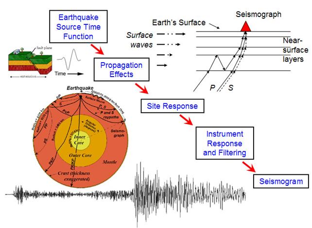
Figure 18. Schematic
illustration of the factors that control the character of the recorded
seismogram. Differences in magnitude of
the earthquake are included in the source time function. Both the amplitude and the duration of the
source time function increase with larger magnitude. Depth of focus also significantly affects the
seismogram. For example, as shown
previously, deep focus earthquakes do not generate strong surface waves. Propagation effects are primarily controlled
by source-to-station distance but can also include variability of Earth
structure between the source and the seismograph station.
Earthquake seismograms can usually be recognized by fairly distinctive
characteristics that result from the effects of the source, propagation path
and seismograph response. A list of
several of these characteristics is shown in Figure 19. Many of these distinctive characteristics are
visible on the seismograms included in the catalogs above. With some experience, it is generally fairly
easy to recognize earthquake or explosion seismic sources from background noise
or other noise sources (Figure 20).
Recognition becomes more challenging if the seismic signal is small
(small magnitude event or distant event) and the noise is large (often called
small signal-to-noise ratio or S/N).
Some common noise sources are listed in Figure 21. Examples of seismograph records illustrating
these noise sources are shown in Figures 22 to 30. Microseisms (Figure 24) are almost always
present on seismographs although on relatively quiet days the microseismic
noise can have very small amplitudes. For
small or distant events, large microseisms can make the identification of the
first arrival on a seismogram uncertain.
An example of this effect is seismogram P in sections 3 and 4
above. For local and regional events, a
high pass filter can be used to enhance the S/N for microseismic noise.
Figure 19. Distinctive
characteristics of seismograms.
Figure 20. An earthquake
seismogram and noise signals.

Figure 21. Some common noise sources. (“Microseisms are weak, almost continuous background seismic waves or Earth “noise”.
They can only be detected by seismographs. They are often caused by surf, ocean
waves, wind, or human activity,”[ Bolt, 2004].
Microseisms usually look very sinusoidal and have a characteristic
period of about 4-6 seconds. )
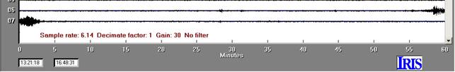
Figure 22. Comparison of quiet
day and noisy day background noise levels.
Both records were plotted with a gain factor of 30.
Figure 23. Comparison of
background noise levels for a seismically quiet day (upper trace, 7/2/04,
Figure 22) and a noisy day (lower trace, 9/29/04, Figure 22) for WLIN AS-1
records. The seismograms are plotted
with the same amplitude scale. The quiet
day seismogram has maximum amplitudes of about 3 digital units. The noisy day seismogram has maximum
amplitudes of about 20 digital units.
Background noise amplitudes as large as 60 digital units (twenty times the quiet day noise levels)
have been observed demonstrating the significance of the noise level on
detection and quality of the recorded signals, particularly from small or
distant earthquakes.
Figure 24. Local high winds (upper
record) can generate fairly large noise signals on the seismograph. Wind noise generally is of higher frequency
(shorter periods) than microseismic noise.
Microsesimic noise (lower record) is usually in the 4-6 s period range.
Figure 25. Microseismic noise
generated by Hurricane Ivan (upper record) and local electronic noise (lower
record). Note that although the
electronic noise signals have long duration in this case, the other
characteristics of the signal are not similar to an earthquake seismogram.
Figure 26. Spike noise (upper
record) and footstep noise (lower record; walking with about 2 meters of the
seismometer).
Figure 27. Close-up of footstep
noise.
Figure 28. Partial AmaSeis
screen image showing an earthquake on 2/24/01.
Figure 29. Extracted seismogram
from the record shown in Figure 28. The
“dropout” is a single point with an amplitude of about -2000 that distorts the
scaling of the seismogram.
Figure 30. Extracted seismogram
shown in Figure 29 after median filter was applied using the AmaSeis filter
tool. The dropout spike has been removed
without significantly distorting the seismogram (in this case, a fairly noisy
seismogram).
![]()
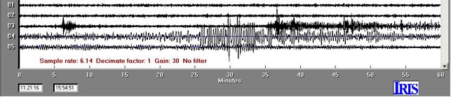
11. Mystery events: Below are twelve “mystery events” (labeled M1 through M12) that are
selected to provide experience in recognizing earthquake seismograms on the
AmaSeis 24-hour screen, making a rough estimate of epicenter-to-station
distance (local, regional, distant or very distant events – these last two
descriptors are sometimes called “teleseisms”), determining distance more
accurately using the S minus P method, and calculating magnitudes. For each event, there is a partial screen
display so that one can see what the seismogram looks like on the “standard”
24-hour AmaSeis screen. All screen
displays have a gain of 30.
M1 Event.
M2 and M3 Events.
M4 Event.
M5 Event.
M6 Event.
M7 Event.
M8 Event.
M9 Event.
M10 Event.
M11 Event.
M12 Event.
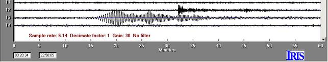
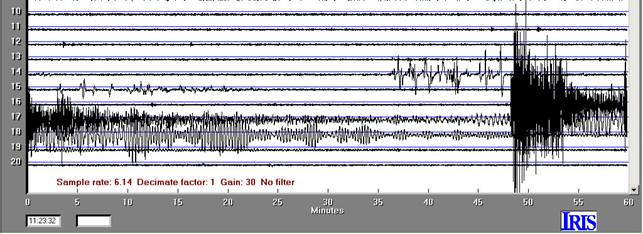
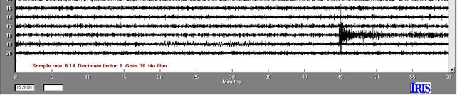
In the figures below, the twelve mystery events are displayed as
individual 60-minute seismograms using the 3-trace plotting capability in
AmaSeis. Each trace is scaled
individually and the amplitude scales on the left display the AS-1 amplitudes
for each trace. Individual seismograms
for each mystery event are available for download (sac format) using the links
given in Table 8.
For each event, one can examine the screen display and the extracted
seismograms and try to determine as much about the event as possible by simple
visual analysis. To gain experience with
this skill, a useful approach is to compare the mystery event with the seismograms
in the catalogs (by distance, by depth and by magnitude) that are provided
above. For example, one can make a rough
estimate of the distance from duration and signal character and observe whether
prominent surface waves are present or not which could suggest the depth of
focus of the event.
Next, use the seismograms downloaded from Table 8 to further analyze
the event. In this step, one can filter
the seismogram and use the AmaSeis tools such as the travel time tool to
determine the distance from the S minus P times and measurements of amplitudes
to calculate magnitude estimates. In
some cases, it is also possible to further identify additional phases in the
seismograms that are of interest for understanding seismic wave propagation in
the Earth or estimating the depth of focus of the earthquake. The parameters column in Table 8 suggests the
most prominent seismogram or earthquake attributes that can be determined from
analysis of the seismograms.
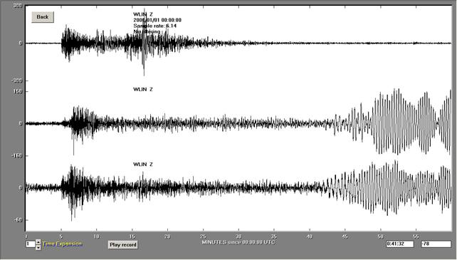
M1, M2 and M3 (top to
bottom) Seismograms.
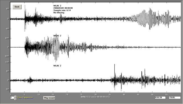
M4, M5 and M6 (top to
bottom) Seismograms. Seismogram M6 is
the smaller event near the beginning of the lower trace.
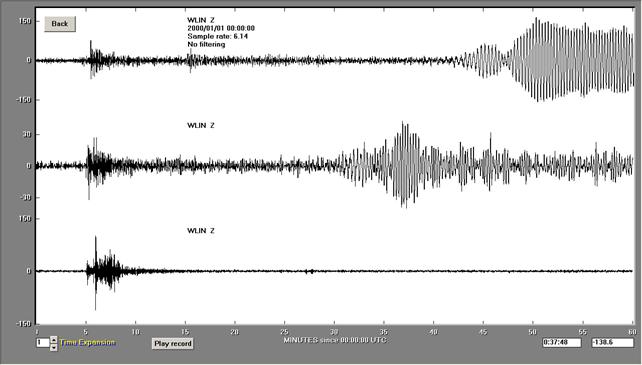
M7, M8 and M9 (top to
bottom) Seismograms.
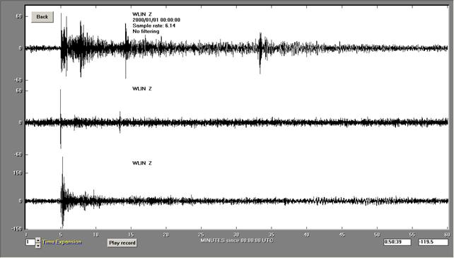
M10, M11 and M12 (top
to bottom) Seismograms.
Table 8. Seismogram download
files for mystery events.
1 In general, low pass filtering (suggested cutoff periods are 2, 5, or
10 s) of teleseismic (distant) seismogram helps enhance the S arrival and
allows one to see the change in frequency that is often associated with the S
phase. Therefore, accurate determination
of the S minus P (S-P) time for many of these seismograms is improved by low
pass filtering (LP).
2 Correctly identifying the S arrival for this seismogram is
challenging. Try the 10 s period LP
filter. Challenge question: What are the
strong arrivals ~3 min. and 45 s after P and ~12 min. and 26 s after P? (Hint: Examine the travel time curves shown
in Figures 5 or 6.)
3 For this seismogram, try using a High Pass (HP) filter with a cutoff
of 1 s to better see the phases.
4 For this seismogram, try using a LP filter with a cutoff of 2 s to
better see the phases.
5 For this seismogram, try using a LP filter with a cutoff of 5 s to
better see the phases. What is the
strong arrival ~2 min. and 45 s after P?
6 For this seismogram, the pP depth phase is present and can be used to
estimate depth of focus using the AmaSeis travel time curve tool.
![]()
Bolt, B.A., Earthquakes and Geological Discovery, Scientific American Library,
W.H.
Bolt, B.A., Earthquakes, (5th edition; similar material is included
in earlier editions), W.H.
Shearer, P. M.,
Introduction to Seismology,
Mystery event information (Excel file of hypocenter information and links to correct time seismograms) is available for viewing with a browser (html file) and for downloading as an MS Word document or PDF file at the following locations:
http://web.ics.purdue.edu/~braile/edumod/as1lessons/InterpSeis/MysteryEqs.htm
http://web.ics.purdue.edu/~braile/edumod/as1lessons/InterpSeis/MysteryEqs.doc
http://web.ics.purdue.edu/~braile/edumod/as1lessons/InterpSeis/MysteryEqs.pdf.
Information on the early history of seismographs can be found at: http://earthquake.usgs.gov/learning/topics/seismology/history/history_seis.php.
Additional references on Seismogram interpretation:
Kulhanek. O., Anatomy of Seismograms 1990 Elsevier.
Manual of Seismological Observatory Practice (1979 edition): http://www.seismo.com/msop/msop79/rec/rec.html#aa30 and http://www.seismo.com/msop/msop79/msop.html.
Ruth B. Simon, Earthquake Interpretations, A manual for reading seismograms, William Kaufmann Inc. 1981
![]()
[1]  Last
modified January 15, 2007
Last
modified January 15, 2007
The web page for
this document is:
http://web.ics.purdue.edu/~braile/edumod/as1lessons/InterpSeis/InterpSeis.htm
Partial funding for this development provided by the National Science Foundation.
ã Copyright 2006. L. Braile. Permission granted for reproduction for non-commercial uses.