|
The
AS-1 Seismograph –Magnitude Determination L. W. BraileÓ, November, 2002 Updated April
30, 2006 |
|

Estimating Earthquake Magnitude from AS-1 Seismograms: Magnitude
is an estimate of the energy release or size of an earthquake. Magnitude estimates are calculated from the
amplitude of wave energy on a seismograph adjusting for the distance of the
seismograph station from the earthquake (seismic waves spread out and are
absorbed during propagation and thus generally become smaller at greater
distances from the earthquake epicenter) and the amplification of the signal by
the seismograph. Magnitude formulas
have been developed for different types of seismographs (usually dependent on
the frequency response of the seismograph) and different type of seismic
arrivals (body waves and surface waves).
Usually, the formulas are valid for a certain range of epicenter to
station distances or region (for example, Richter magnitude was developed for
neic.usgs.gov/neis/general/handouts/general_seismicity.html
www.seismo.unr.edu/ftp/pub/louie/class/100/magnitude.html
lasker.princeton.edu/ScienceProjects/curr/eqmag/eqmag.htm
http://www.eas.slu.edu/People/CJAmmon/HTML/Classes/IntroQuakes/Notes/earthquake_size.html
http://www.seismo.com/msop/nmsop/03%20source/source4/source4.html
Currently, in an effort
to reduce confusion about earthquake magnitudes and use the most reliable measure
of earthquake size, most magnitudes reported by the US Geological Survey (http://earthquake.usgs.gov)
are labeled “Magnitude” or “M” and are moment magnitude (sometimes
referred to as Mw) determinations (when available). However, traditional magnitude determinations
such as body wave magnitude (mb), surface wave magnitude (MS) and Lg wave
magnitude (mbLg) are also reported in USGS earthquake catalogs. Determinations of magnitude for these
magnitude definitions can be made using data from the AS-1 seismograph.
The procedure for
determining magnitude from seismograms recorded by the AS-1 seismograph is:
From
the AmaSeis software, determine the approximate arrival time of the
earthquake. If possible, pick the P and
S arrivals (filtering the seismogram may help in the identification of the S
wave) and estimate the distance using the travel time curve tool. Using the selection tool, zoom in on the P
wave (extract the early part of the seismogram; the time expansion tool at the
bottom left of the screen may also be useful for zooming in on the P arrival)
and determine the maximum amplitude (zero to peak, in counts) and the
approximate period of the P wave. Use
the largest amplitude of the P wave. The
P arrival may include energy that occurs during the first approximately 10 s of
the record. Often, a distinct secondary
P phase (such as pP or PP) will be present after the first P arrival. Estimate the period by measuring the time in
seconds between two successive peaks or troughs of the signal. A millimeter scale held up to the screen is
useful to this measurement. Next, using
the selection tool, extract the early (usually largest) part of the surface
wave signal (the surface waves will usually be distinguished by their much
lower frequency) on the seismogram and determine the maximum amplitude (zero to
peak, in counts) of the surface wave arrival that is near 20 s period. Note the period of the surface wave where
your amplitude measurement is made.
1.
Go to the USGS
earthquake search web site (neic.usgs.gov/neis/epic/epic.html)
or the IRIS earthquake search site (http://www.iris.washington.edu/, select Event Search under the Quick Links menu at
left side of screen) or, for recent events, to the USGS earthquake site (http://earthquake.usgs.gov,
select Latest Quakes and then NEIC Current Earthquake Information) or the IRIS
Seismic Monitor tool, www.iris.edu) and find
and record the “official” origin time, location (latitude and longitude; note S
latitudes and W longitudes are negative; and depth) and magnitude. Several magnitude estimates may be available
(for events that occurred at least a week earlier, the IRIS event search tool
can be used to find different magnitude estimates; for example, the primary
magnitude reported may be Mw (moment magnitude) which cannot be estimated from
AS-1 record, but mb and MS magnitude may be reported later). The IRIS sites also provide a brief
geographic description of the earthquake location that is often useful.
2.
Go to the USGS
travel time and distance calculation site (http://neic.usgs.gov/neis/travel_times/) and calculate the distance from your seismograph
station to the earthquake epicenter by entering the latitudes and longitudes of
the event and the station into the web site form. If you don’t know the latitude and longitude
of your station, you can view a topographic map and use the tools to find a
specific location at www.maptech.com
(click on Online Maps select the Map Server, then enter city and state in the
boxes and click go; select correct map from list if list of possible maps
appears; choose DD.DD in coordinates window to the left of the displayed
topographic map; place cursor on location of interest; read the latitude and
longitude of the cursor location from the display to the left of the map). For interest, you can compare the calculated
distance (in degrees, geocentric angle) with the distance that you determined
from the P and S arrivals (S – P time) in AmaSeis.
3.
Using the
Amplitude, distance, period and displacement amplification (read from the table
provided in the computer code below) data, calculate the magnitude estimate(s)
for the earthquake. The calculations can
easily be made with a hand calculator or one can write a simple computer
program such as the Matlab code shown below.
Note that valid data from the magnitude formulas will usually be
restricted to certain distance ranges.
Compare the magnitudes determined from your AS-1 seismogram with the
official magnitude estimates.
Magnitude formulas, a
table of amplification information for the AS-1 seismograph (amplification
versus period) and a sample Matlab computer code that uses the amplitude,
distance, period, displacement amplification data and the magnitude formulas to
calculate magnitude estimates is shown below:
% Calculate magnitudes for AS-1
Seismograms
% L Braile,
%----------------------------------------------------------------
%
% a = amplitude (zero to peak) in
counts of the arrival on AS-1 seismogram
% D = distance in degrees
(geocentric angle; one degree = 111.19 km on surface)
% T = period (s) of the arrival
(measure by distance between two peaks)
% Velamp = velocity amplification
of AS-1 in counts/micron/s
% Disamp = displacement
amplification of AS-1 in counts/micron
% Disamp = Velamp*2*pi/T
% A = displacement amplitude =
a/Disamp (microns)
%
%----------------------------------------------------------------
% Table of amplification versus
period for the AS-1 seismograph
%----------------------------------------------------------------
%
Period, T Frequency Vel. Amplification Displ. Amplification
% (s)
(Hz) (counts/micron/s) (counts/micron)
%----------------------------------------------------------------
% 1 1 12 75
% 1.5 0.667 22 92
% 2
0.5 28 88
% 3 0.333 28 59
% 5 0.2 22 28
% 10 0.1 9 5.7
% 15 0.0667 4 1.7
% 20 0.05 2 0.63
% 30 0.333 0.7 0.15
% 50 0.02 0.15 0.019
% 100 0.01 0.02 0.0013
%----------------------------------------------------------------
% Change a, D, T, and Disamp for
each calculation.
% Read Disamp from table above for
appropriate period, T.
% Use magnitude estimate (mb, MS,
mbLg1, or mbLg2) appropriate to data.
% Note distance ranges and approximate
period information for each
% magnitude formula. Magnitude equations are from Bolt (1999) for
mb
% and USGS/NEIC for MS and
mbLg. Amplification factors are
% from AS-1 calibration data provided
by Tim Long (Georgia Tech;
% http://quake.eas.gatech.edu/MagWeb/CalReptAS-1.htm.
% Bob Hutt (USGS, Albuquerque)
clarified the use of the amplification
% factors in the magnitude
formulas.
%----------------------------------------------------------------
a=28;
D=45.07;
T=20;
Disamp=0.63;
A=a/Disamp;
mb = log10(A/T) + 0.01*D + 5.9 % 25 deg <
D < 90 deg; T~1-3 s
MS = log10(A/T) + 1.66*log10(D) + 3.3 % 20 deg
< D < 160 deg; T~20 s
mbLg1 = log10(A/T) + 0.90*log10(D) +3.75 % 0.5 deg
< D < 5 deg; T~1 s
mbLg2 = log10(A/T) + 1.66*log10(D) +3.3 % 5 deg <
D < 30 deg; T~1 s
%----------------------------------------------------------------
Magnitude Calculator: A new online magnitude calculator for the AS-1 seismograph is available at: http://web.ics.purdue.edu/~braile/edumod/MagCalc/MagCalc.htm. The calculator can be used to calculate mb, MS and mbLg magnitudes from AS-1 amplitude data. The calculator uses the same equations that are programmed in the Matlab code shown above. It is also possible to use these equations to perform the calculations with a simple electronic calculator “by hand”.
AmaSeis Updates: A new version of AmaSeis (http://www.geol.binghamton.edu/faculty/jones/) includes the ability to easily determine time and amplitude on an extracted seismogram. For example for the September 25, 2003 M8.0 Hokkaido, Japan earthquake (Figure 1), the extracted seismogram (after selection with the cursor on the 24-hour screen display or from opening a previously saved .sac file) is shown with an actual (UTC) time scale below the seismogram. In addition two small windows appear in the lower right hand corner of the screen. The first of these windows displays the actual UTC time (assuming that the computer’s clock has been synchronized with UTC time) of the position of the cursor (horizontal position on the screen) and the second window shows the amplitude (in digital units) of the cursor position (vertical position on the screen). These tools can be used to easily measure times of arrivals on the seismogram and amplitudes of the arrivals for magnitude calculation. When measuring amplitudes, it is necessary to not the position of the approximate zero line on the seismogram. If the recorded signals are centered on the zero line, then no adjustment is necessary. If signals are offset from the zero line, then the amplitude of the peak used for the magnitude measurement should be measured from the position of the signal zero line and needs to be adjusted by the amount of the zero line offset (usually a small number of digital units).
Examples of magnitude calculations using the AS-1 online magnitude calculator and the AmaSeis time and amplitude measuring tool are shown in Figures 1, 2 and 3.
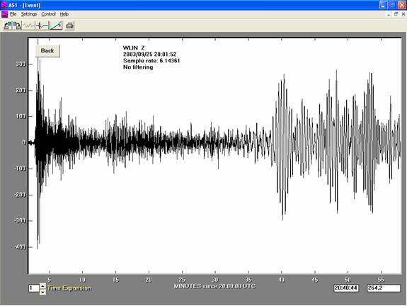
Figure
1. AmaSeis seismogram for the M8.3
September 25, 2003 Hokkaido,
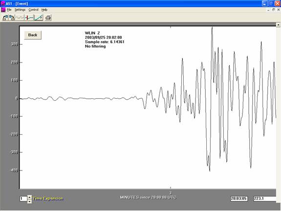
Figure
2. Enlarged (selected in AmaSeis)
seismogram for the P wave arrival for the M8.3
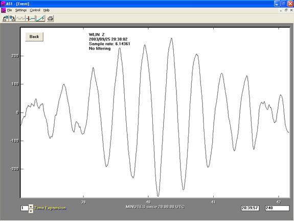
Figure
3. Enlarged (selected in AmaSeis)
seismogram for the ~20 s surface wave arrivals for the M8.3
Example Magnitude Calculations for AS-1 Seismograms: Examples of AS-1 seismograms and magnitude
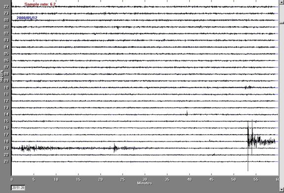
calculations are given below. Figure 4
shows a 24 hour AS-1/AmaSeis screen display of seismic data including the
August 4, 2000 Sakhalin Island earthquake recorded in West Lafayette,
Indiana. Prominent first arriving P
waves and surface waves are visible. The
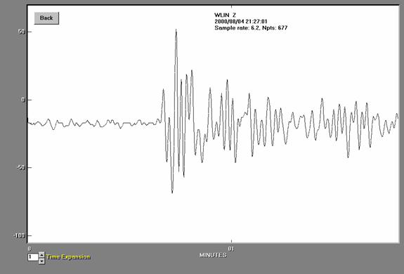
extracted seismogram for the
a = 70 counts,
T = 2 s,
D = 81.08 degrees,
Dispamp = 88
counts/micron, (so A = a/Disamp = 70/88 microns),
and the body wave
formula: mb = log10(A/T) +
0.01*D + 5.9,
the
magnitude is mb = 6.3. This magnitude is
the same as the official, USGS magnitude of mb = 6.3.
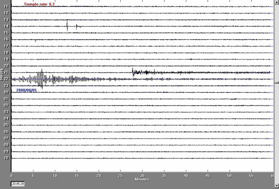
Figure
4. AmaSeis 24 hr. record including the
Aug.t 4, 2000
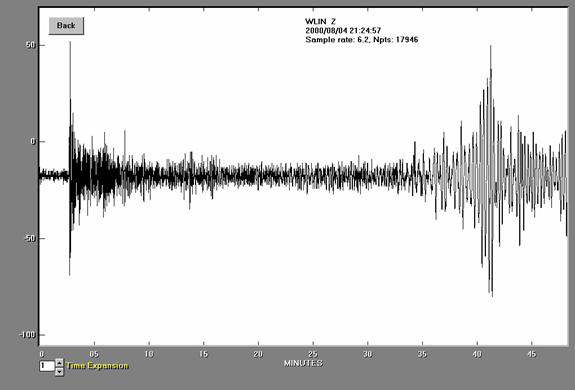
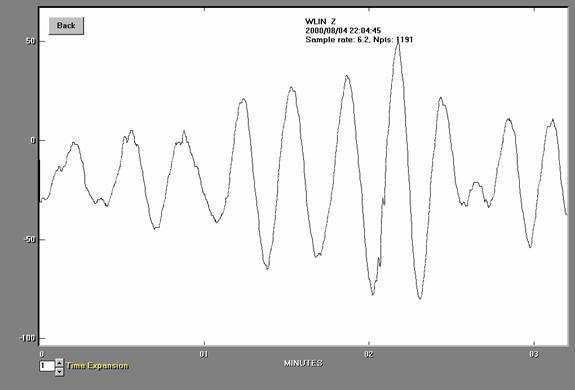
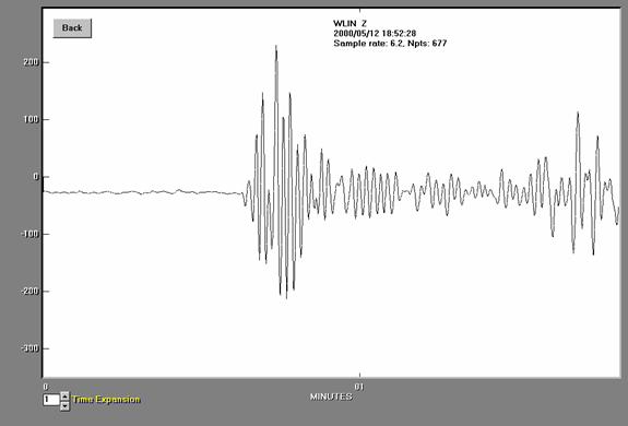
Figure 5.
Seismogram for the
Figure
6. Seismogram for the
A
close-up view of the surface waves for the
a = 60 counts,
T = 20 s,
D = 81.08 degrees,
Disamp = 0.63
counts/micron, (so A = a/Disamp = 60/0.63 microns),
and the surface wave
formula: MS = log10(A/T) +
1.66*log10(D) + 3.3,
the calculated magnitude
is MS = 7.1, the same as the USGS magnitude of MS = 7.1.
Figure
7. Seismogram for the
An additional example of
body wave and surface wave magnitude calculations is provided by the
seismograms for the
Figure
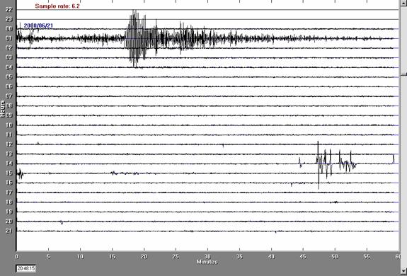
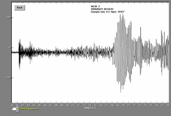
8. AmaSeis 24 hour seismic record
including the June 21, 2000
A
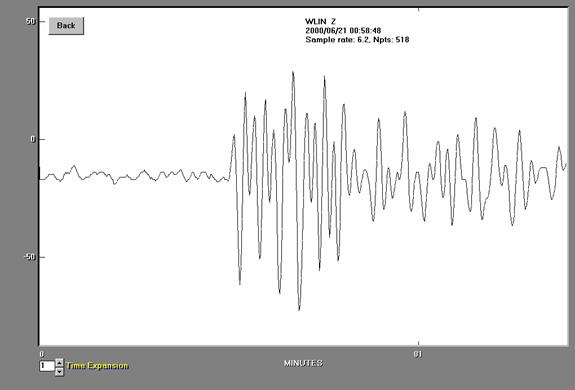
close-up view of the P wave for the
a = 60 counts,
T = 1.5 s,
D = 44.23 degrees,
Disamp = 92
counts/micron, (so A = a/Disamp = 60/92 microns),
and the body wave
formula: mb = log10(A/T) +
0.01*D + 5.9,
the
magnitude is mb = 6.0 compared to the USGS magnitude of mb = 6.1.
Figure
9. Seismogram for the
Figure
10. Seismogram for the
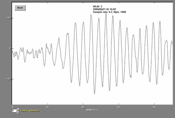
A
close-up view of the surface waves for the
a = 120 counts,
T = 15 s,
D = 44.23 degrees,
Disamp = 1.7
counts/micron, (so A = a/Disamp = 120/1.7 microns),
and the surface wave
formula: MS = log10(A/T) +
1.66*log10(D) + 3.3,
the calculated magnitude
is MS = 6.7 compared to the USGS magnitude of MS = 6.6.
Figure
11. Seismogram for the
An example of calculating
magnitude for a deep focus earthquake (in which surface waves are generally
very small so that the surface wave magnitude formula cannot be used) is shown
in Figures 12, 13 and 14. The formula
used here and in the Matlab code above is a simplified formula in which no
correction is made for the depth of the earthquake. Often (including the USGS magnitude
calculations), mb calculations for deeper earthquakes include a correction for
the effect of depth. A description of
this procedure and the graph showing correction factors is given at: http://www.seismo.com/msop/nmsop/03%20source/source4/source4.html. Figure 12 shows an AmaSeis screen display for
the
Figure
12. AmaSeis 24 hour seismic record
including the May 12, 2000
Figure
13. Seismogram for the deep-focus
event
is shown in Figure 14. Using the
following data for the P wave arrival:
a = 150 counts,
T = 2 s,
D = 66.48 degrees,
Disamp = 88
counts/micron, (so A = a/Disamp = 150/88 microns),
and the body wave
formula: mb = log10(A/T) +
0.01*D + 5.9,
the magnitude is mb = 6.5 compared to the USGS magnitude of mb = 6.2.
Figure
14. Seismogram for the
The calculation of the
mbLg magnitude can be illustrated with the regional event from Figure 15 (
a = 25 counts,
T = 1.0 s,
D = 2.63 degrees,
Disamp = 75
counts/micron, (so A = a/Disamp = 25/75 microns),
and the mbLg formula: mbLg = log10(A/T) + 0.90*log10(D) +3.75,
the
magnitude is mbLg = 3.7 compared to the USGS magnitude of mbLg = 3.9.
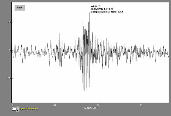
Figure
15. AS-1 seismogram recorded at West
Lafayette, Indiana from an earthquake located near Evansville, Indiana,
December 7, 2000. The earthquake
epicenter was about 292 km away from the seismograph and had a magnitude of
about 3.9 (mbLg). Microseisms of about 3-6
second period are visible before the first arrival (the compressional or P wave)
that is located at about 1.1 minutes (relative time). The S (Shear) wave and surface waves are the
largest arrivals following the P wave.
A comparison of
magnitudes calculated from AS-1 seismograph data using the procedures described
here with USGS magnitudes is shown in Figure 16. If the magnitude estimates agreed perfectly,
the data would plot on the diagonal line. This comparison suggests that earthquake
magnitudes can be determined from AS-1 seismograph records with an accuracy of
about +/- 0.5 magnitude units (95% confidence limits). Some variation in magnitude estimates is
expected because: seismograph stations are located on different geological
materials (variation in site response); the radiation pattern of seismic waves
generated by earthquakes (because seismic waves are caused by release of energy
associated with slip along a fault plane with a specific orientation, energy is
not propagated equally in all directions); there is variation in the
amplification of seismographs; and amplitude and period measurement on the
seismogram is subject to some interpretation and error.
Although we cannot
calculate moment magnitude (Mw or simply, M) from AS-1 seismograms, the AS-1
magnitudes (mb, MS and mbLg) provide reasonably accurate estimates of Mw
(Figure 17).
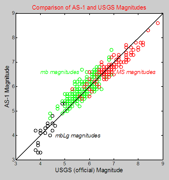
Figure
16. Comparison of magnitudes for
earthquakes recorded by an AS-1 seismograph (calculated using the procedures
and formulas given in the text) and the USGS magnitude determinations for the
earthquakes. Data form January 1, 2000 to
March 31, 2006.
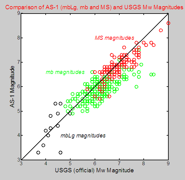
Figure 17. Comparison of AS-1 magnitudes (mbLg, mb and MS) with USGS Mw magnitudes.
References:
Bolt,
B.A., Earthquakes and Geological
Discovery, Scientific American Library, W.H.
Bolt,
B.A., Earthquakes, (4th
edition), W.H. Freeman & Company,
Return to
Braile’s Earth Science Education Activities page
Related
Pages:
The AS-1
Seismograph – Installation and Calibration
The AS-1
Seismograph – Operation, Filtering, S-P Distance Calculation, and Ideas