Earth’s Interior Structure - Seismic Travel Times in a Constant Velocity Sphere


(L. BraileÓ, December, 2000)

http://web.ics.purdue.edu/~braile


Introduction:  Using simple calculations of the travel times of seismic waves in a constant velocity, spherical Earth and comparison of the travel times with observations for the real Earth, we find that the Earth’s interior is not homogeneous.  Examination of the travel time data and calculations provides suggestions about the actual nature of the Earth’s interior structure.

Educational Objective:  Provide experience with graphing, calculations and graphical analysis.  Infer the structure of the Earth’s interior and gain experience with the methods used to study Earth structure.  Optionally, provide an opportunity to make calculations using a calculator from an equation, or to write a computer program to perform seismic travel time calculations.

Possible Preparatory Lessons/Activities:

Seismic wave propagation

Elasticity

Materials:

2 11” x 17” sheets of photocopy paper

metric ruler

calculator

pencil or pen

40 cm long piece of string

protractor

scotch tape

copies of figures


Procedure:


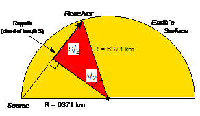
1.   Draw a cross section of half of the spherical Earth using a scale of 1:25,000,000 on the two sheets of paper taped together along the long side (Figure 1).  Use the string with a loop at one end to draw the semi-circle arc with a radius of 25.5 cm to represent the Earth’s surface in the cross section diagram.  Alternatively, a template (Figure 2) is provided to make the half-sphere model.  Copy the template (one half of figure at a time onto an 11x17 piece of paper using 200% enlargement.  The two halves can then be taped together.


2.   Draw raypaths associated with geocentric angles (a measure of distance from a source [earthquake] to a receiver [seismograph station]) of 40°, 80°, 120°, 150° and 180°.  Use the protractor to measure the angles.  One angle and raypath is shown in Figure 1 as an example.


3.   Measure the distance (in cm, using the metric ruler) from source to receiver along the raypaths for each of the angles and write the result in Table 1.  Convert these measurements to units of km for the real Earth by multiplying by 250 (accounting for our scale factor of 1 cm = 250 km or 1:25,000,000 in the scale model diagram) and write these numbers in the third column of the table.  Determine the travel times for each raypath assuming a constant velocity of 11 km/s (divide length of raypath in km by velocity in km/s).  Convert these times to minutes by dividing by 60.  (These calculations could have been made more precisely by deriving a formula for the length of a chord of a circle using the geometry illustrated in Figure 3.  However, the graphical solution is adequate to illustrate the concept of travel times through the Earth and is more concrete.  We will use the formula which follows from the diagram in Figure 3 in the calculation of travel times using a computer program.  You could also try other constant velocities, such as 10 km/s or 12 km/s, to see if the calculated travel times better fit the observed data.)


Table 1.  Calculation of travel times for raypaths in a spherical, constant velocity Earth at various distances (geocentric angle).


Geocentric

Angle

D (degrees)

Length of

Raypath

measured on

diagram

(cm)


Actual

raypath length

(km)


Travel

Time

(s)


Travel

Time

(min)


40


80


120


150


180


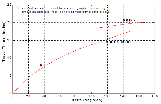
4.   Plot the calculated travel times at the five distances (place a dot at the distance and location given by the data in columns 1 and 5 of Table 1 on the graph shown in Figure 4.  Draw a smooth curved line through the calculated travel times (from the graphical calculations, Table 1) beginning at zero distance (Delta) and zero time.  Observed travel times for the compressional wave are plotted as solid lines.  These lines correspond to three different phases (different paths through the Earth), but for now are simply used for a comparison with the calculated times.  Do the observed and calculated times differ significantly?  What does this imply about our assumption that the Earth’s interior might consist of a constant velocity of 11 km/s?


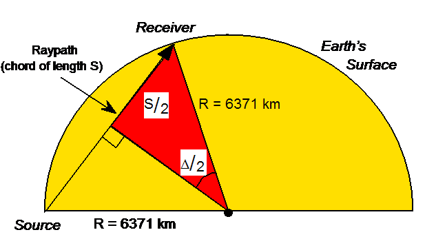
5.   We can calculate the travel times in a homogeneous Earth more precisely (and thus compare observed and calculated travel times at all distances) using an equation corresponding to the geometry shown in Figure 3.


      From the shaded triangle in the diagram in Figure 3, we have


                                                                                                    (1)


or,


                                                                                                   (2)


(R and S are in kilometers and D is in degrees)


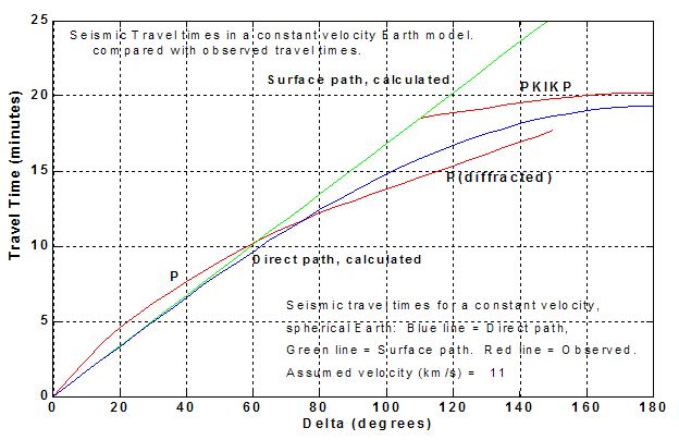
      from which the length of the raypath can be calculated for any distance (geocentric angle), D.  The travel times for a constant velocity Earth can then be calculated by dividing by the assumed velocity.  In order to compare the observed travel times with other possible raypaths, we also calculate the travel times for the path along the surface of the homogeneous Earth.  For this path, the distance is just D in degrees, or D multiplied by 111.19 km/degree to obtain the distance in km, which can be used to determine travel time by dividing by velocity.  A computer program (Table 2) to calculate and plot the travel times was prepared using MATLAB* .  The calculations could be made by writing a program in any computer language.  The results of the calculations from the program are illustrated in a travel time graph (Figure 5) and in the tabular output of the program (Table 3).


Questions:


Examine the observed and calculated travel times shown on the graph (Figure 5) and answer the following questions.


1.   Do the observed travel times differ significantly (discuss what differ significantly means in this analysis; compare differences with the expected experimental error in the travel times) from the calculated times for the surface and direct paths?  (The time of arrival of seismic waves at a seismograph station can usually be determined with an accuracy of better than 1 second.)


2.   If the Earth is homogeneous but we selected a different velocity than 11 km/s, could we obtain an adequate fit between the observed and calculated travel times?  Why or why not?  (Note that we could easily try many different velocities using the graphical solution, calculations using a calculator and the formula given above for determining the raypath length, S, or by using the computer program.)


3.   Now that we know that the Earth’s interior cannot consist of a constant velocity, we use the travel time information to make additional inferences about the velocity structure of the interior.  Examine the raypaths that you constructed using the graphical analysis.  By comparing the distance ranges where the observed and calculated travel times (for the P and P diffracted phases) differ significantly in Figure 5 with the “depth penetration” of the corresponding raypaths in the hand-plotted graph, can you infer the relative velocity (compared to our 11 km/s assumption) of the actual Earth’s interior for the shallow (about 0 to 1500 km depth) and deeper (greater than 1500 km depth) regions of the Earth?  In other words, is the assumed constant velocity of 11 km/s too high or too low for the shallow or deep Earth?


4.   What causes the travel time curves to “flatten” so strongly in the distance range of about 160 to 180 degrees?


5.   From the simple analysis that we have performed, we can infer that Earth’s interior has a velocity structure in which the velocity varies with depth.  How could we determine if the velocity also varies laterally (with location)?


Additional Information:


1.   Examine Chapter 6 of Bolt (1993) to learn more about the actual velocity structure of the Earth’s interior and how this information has been obtained, both historically and utilizing modern and much more extensive observations and techniques.


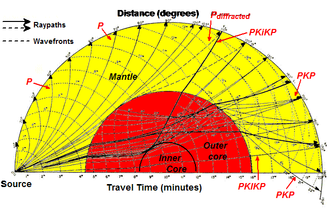
2.   The raypaths for compressional waves in a more accurate Earth model are shown in Figure 6.


Possible Follow-Up Lessons/Activities:


Earth’s Interior Structure (Scale model “slice” through the Earth)

Reflection and Refraction

SEISMIC WAVES Program

Earthquake location techniques


References:


Bolt, B.A., Earthquakes and Geological Discovery, Freeman, San Diego, California, 229 pp., 1993.


Richter, C.F., Elementary Seismology, Freeman, San Francisco, California, 1958.


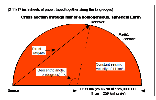
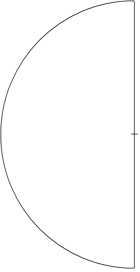
Figure 1.  Cross section through half of a homogeneous, constant seismic velocity, spherical Earth.  Sample seismic raypath from a surface source to a receiver at a distance of D degrees geocentric angle (one degree corresponds to 111.19 km, measured along the surface, for a 6371 km sphere) is shown by the heavy line.  For a graphical construction of this model and measuring the distance along raypaths corresponding to various geocentric angles (distances), the half circle can be drawn at a scale of 1:25,000,000 on two sheets of 11x17 inch paper taped together.


Figure 2.  Template for making a 1:25 million scale model of a cross section through the Earth.  Photocopy at 200% enlargement (or set the enlargement to the percentage that will make the radius of the final half-circle 25.5 cm) onto 11 x 17 inch paper; then tape together to make a half circle with radius of 25.5 cm.  Photocopy the top one quarter of the circle on one sheet of paper (widthwise) and the lower one quarter of the circle on another.  Be sure that the tic mark identifying the center of the half circle is visible on both sheets of paper.  Trim to make two quarter circles and tape together.


Figure 3.  Diagram illustrating the calculation of the length of a chord, S, corresponding to a geocentric angle of D degrees.


Figure 4.  Graph for plotting calculated travel times.


Figure 5.  Travel times of observed and calculated P waves.


Figure 6.  Raypaths and wavefronts for selected primary (compressional) wave phases which travel through the Earth.  The travel times (in minutes) along the raypaths and the corresponding wavefronts (short dashed lines; lines or surface of equal travel time) are given by the small numbers adjacent to the wavefronts.  The raypaths are perpendicular to the wavefronts and represent the direction that a specific point on the wavefront is propagating.  The raypaths in this real Earth model are curved because the seismic wave velocity varies with depth.  Note the strong refraction (bending) of the raypaths and wavefronts caused by the velocity change across the core-mantle boundary.  The primary wave types (phases) illustrated in this diagram are:

P                      Raypaths for waves which travel through the mantle with a reltively direct path; 0°-103° distance range.

Pdiffracted       Raypaths for waves which travel through the mantle and are diffracted at the core-mantle boundary by the reduced outer core velocity; 103°-150° distance range.

PKP                 Raypaths for waves which travel through the mantle, are strongly refracted at the core-mantle boundary and travel through the outer core; 110°-187° distance range.

PKIKP             Raypaths for waves which travel through the mantle, the outer core and the inner core; 110°-180° distance range.

PKiKP              Raypaths for waves that are reflected from the inner core.  In more recent models of the Earth's interior, the PKiKP arrivals are observed for distances less than about 120°.


Table 2.  Program (written in MATLAB code) to calculate and plot seismic travel times in a spherical, constant velocity Earth.  Observed P-wave travel time data for the real Earth are also included in the plot.  Comments begin with a percent sign (%).  The plot produced by the program is given in Figure 5.  Calculated data from the program are shown in Table 3.


%  Program to calculate and plot seismic travel times

%  in a spherical, homogeneous velocity Earth. 

%

%  Program written in Matlab code.

%  (L. Braile, Purdue University, 5/7/96; updated 12/9/00)

%

%---------------------------------------------------------------

R = 6371;      % radius of Earth (km)

V = 11;        % assumed constant seismic wave velocity (km/s)

%---------------------------------------------------------------

%

%  Calculate travel times along Earth's surface

%

delta = 0:5:180;     % distance in degrees, geocentric angle,

%                    % from 0 to 180 in steps of 5 degrees;

%                    % on the surface, one degree = 111.19 km

delrad = delta/57.2958; % convert degrees to radians

S = R*delrad;        % calculate distance in km along surface

Ts = S/V;            % travel time in seconds

Tm = Ts/60;          % travel time in minutes

%

%---------------------------------------------------------------

% Compute travel times through the Earth's interior (body waves)

%

S = 2*R*sin(0.5*delrad);% calculate length of chords (raypaths) in km

Ti = S/V;               % travel time in seconds

Ti = Ti/60;             % travel time in minutes

%

%---------------------------------------------------------------

% Input observed travel times (min., first arrivals) for comparison

% P and P(diffracted) arrivals.  (0 deg. to 105 deg for P, 105 deg

% to 150 deg. for P(diffracted).  NaN is "not a number" inserted to

% maintain equal size of all arrays and not be plotted on figure.

%

To = [0 1.302 2.467 3.583 4.617 5.447 6.208 6.935 7.635 8.315];

To = [To 8.967 9.590 10.178 10.733 11.257 11.750 12.212 12.642];

To = [To 13.045 13.428 13.807 14.177 14.570 14.964 15.357 15.750];

To = [To 16.144 16.537 16.930 17.324 17.717 NaN NaN NaN NaN NaN NaN];

%

%  PKIKP observed arrivals (110 deg. to 180 deg.)

%

To2 = [NaN*ones(22,1)' 18.553 18.717 18.878 19.040 19.200 19.357];

To2 = [To2 19.508 19.653 19.790 19.908 20.013 20.097 20.153];

To2 = [To2 20.192 20.203];

%

%---------------------------------------------------------------

%  Print matrix of values


%  Table 2. (continued)

format compact

'Table 3.  Travel times for a homogeneous Earth, Velocity (km/s) ='

V

Heading=['    Delta   T surface  T direct  T observed  T(PKIKP) observed',

         '    (deg)     (min)     (min)      (min)          (min)       ']

Data=[delta' Tm' Ti' To' To2']

%

%---------------------------------------------------------------

%  Plot travel time curves for Observed and Calculated arrivals

%

plot(delta,To,'-r','linewidth', 2)     %  Observed P and P(diffracted)

hold on                                %  Keep all lines on plot

plot(delta,To2,'-r','linewidth', 2)    %  Observed PKIKP

plot(delta,Tm,'g','linewidth', 2)      %  Calculated, surface path

plot(delta,Ti,'-b','linewidth', 2)     %  Calculated, direct path

%

%---------------------------------------------------------------

% Label plot

%

set(gca,'fontsize',18,'fontweight', 'bold','linewidth',1)

text(75,-1.9,'Delta (degrees)','fontsize',18,'fontweight','bold')

text(-11,9,'Travel Time (minutes)','rotation',90,'fontsize',18,...

'fontweight','bold')

text(70,6,'Seismic travel times for a constant velocity,',...

'fontsize',16)

text(70,4.5,'spherical Earth:  Blue line = Direct path,',...

'fontsize',16)

text(70,3,'Green line = Surface path.  Red line = Observed.',...

'fontsize',16)

vel=num2str(V);

text(70,1.5,'Assumed velocity (km/s) =','fontsize',16)

text(131,1.5,vel,'fontsize',16)

text(35,7.9,'P','fontsize',18,'fontweight','bold')

text(118,14.5,'P(diffracted)','fontsize',18,'fontweight','bold')

text(140,20.5,'PKIKP','fontsize',18,'fontweight','bold')

text(64,21,'Surface path, calculated','fontsize',16,'fontweight','bold')

text(60,9,'Direct path, calculated','fontsize',16,'fontweight','bold')

text(5,24,'Seismic Travel times in a constant velocity Earth model.',...

'fontsize',16)

text(5,23,'     compared with observed travel times.',...

'fontsize',16)

%---------------------------------------------------------------

%  Set axis size

axis([0 180 0 25]);

grid on         %  Plot grid lines on graph

hold off

%  End of program

%---------------------------------------------------------------


Table 3.  Travel times for a constant velocity Earth (assumed velocity = 11 km/s).  Output from the computer program given in Table 2.  


  Delta   T surface   T direct   T observed   T(PKIKP) observed

  (deg)     (min)     (min)      (min)          (min)      


         0         0         0         0       NaN

    5.0000    0.8424    0.8421    1.3020       NaN

   10.0000    1.6848    1.6826    2.4670       NaN

   15.0000    2.5272    2.5199    3.5830       NaN

   20.0000    3.3695    3.3525    4.6170       NaN

   25.0000    4.2119    4.1786    5.4470       NaN

   30.0000    5.0543    4.9968    6.2080       NaN

   35.0000    5.8967    5.8054    6.9350       NaN

   40.0000    6.7391    6.6031    7.6350       NaN

   45.0000    7.5815    7.3881    8.3150       NaN

   50.0000    8.4239    8.1591    8.9670       NaN

   55.0000    9.2662    8.9145    9.5900       NaN

   60.0000   10.1086    9.6530   10.1780       NaN

   65.0000   10.9510   10.3731   10.7330       NaN

   70.0000   11.7934   11.0735   11.2570       NaN

   75.0000   12.6358   11.7528   11.7500       NaN

   80.0000   13.4782   12.4097   12.2120       NaN

   85.0000   14.3206   13.0430   12.6420       NaN

   90.0000   15.1629   13.6514   13.0450       NaN

   95.0000   16.0053   14.2339   13.4280       NaN

  100.0000   16.8477   14.7893   13.8070       NaN

  105.0000   17.6901   15.3165   14.1770       NaN

  110.0000   18.5325   15.8146   14.5700   18.5530

  115.0000   19.3749   16.2826   14.9640   18.7170

  120.0000   20.2173   16.7195   15.3570   18.8780

  125.0000   21.0596   17.1247   15.7500   19.0400

  130.0000   21.9020   17.4972   16.1440   19.2000

  135.0000   22.7444   17.8365   16.5370   19.3570

  140.0000   23.5868   18.1418   16.9300   19.5080

  145.0000   24.4292   18.4125   17.3240   19.6530

  150.0000   25.2716   18.6482   17.7170   19.7900

  155.0000   26.1140   18.8484       NaN   19.9080

  160.0000   26.9563   19.0128       NaN   20.0130

  165.0000   27.7987   19.1409       NaN   20.0970

  170.0000   28.6411   19.2326       NaN   20.1530

  175.0000   29.4835   19.2877       NaN   20.1920

  180.0000   30.3259   19.3061       NaN   20.2030


ÓCopyright 2000.  L. Braile.  Permission granted for reproduction for non-commercial uses.

*MATLAB is a technical computing environment for numeric computation and visualization.  It operates on Macintosh, Windows, UNIX and other computing platforms.  MATLAB is distributed by The MathWorks, Inc., Cochituate Place, 24 Prime Park Way, Natick, MA  01760, (508) 653-1415, www.mathworks.com.  A Student Edition of MATLAB is available from Prentice-Hall publishers.