11. Make your

own mapÓ

Lawrence W. Braile,

Professor

Department of Earth and

Atmospheric Sciences

Purdue University

West Lafayette, Indiana

Sheryl J. Braile, Teacher

Happy Hollow School

West Lafayette, Indiana

January 17, 2002

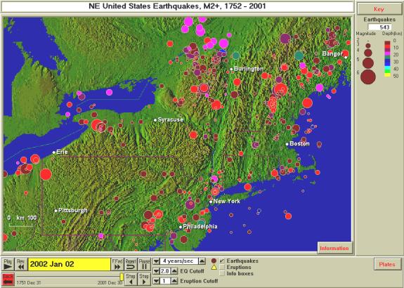
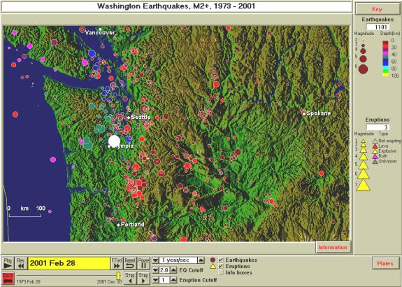
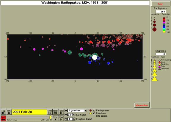
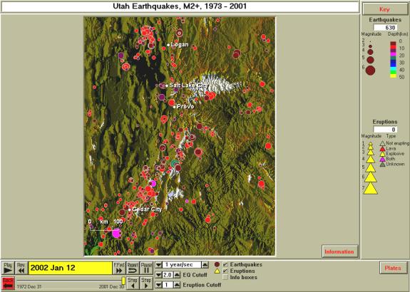
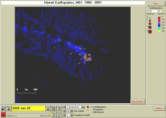
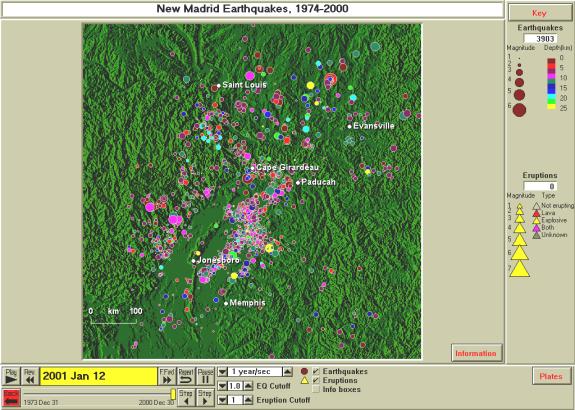
Objective: Use the “Make Your Own Map” option in SeisVolE to create maps of earthquake and volcanic activity for selected areas. Earthquake data from additional catalogs can be selected to produce more detailed maps. Maps can be annotated with titles, a scale and city names to make the map more useful or for special purposes. The “Make Your Own Map” option also allows one to “zoom in” on a map area to see additional detail.

Instructions: The basic “Make Your Own Map” option in SeisVolE is very simple. However, there are many options for modifying the map that you have created, including adding or changing the topographic data used to generate the shaded terrain background map, selecting an alternate earthquake catalog, annotating the map, and saving the view or map image. Because using this option starts from a SeisVolE standard view and potentially involves many changes to data files used and settings, it is possible to corrupt the standard view file. To help prevent this occurrence, it is strongly recommended that you always exit from your “Make Your Own Map” view by using the Back button on the SeisVolE screen (lower left hand corner). If you do find that one or more of the SeisVolE standard views are corrupted, there are two methods of recovery that are described in Teaching Modules 1 and 3. The following section provides instructions and examples for effectively using the “Make Your Own Map” option in Seismic/Eruption.

1. Open the SeisVolE standard view with that contains your area of interest (for example, for a state in the US, open the United States view).

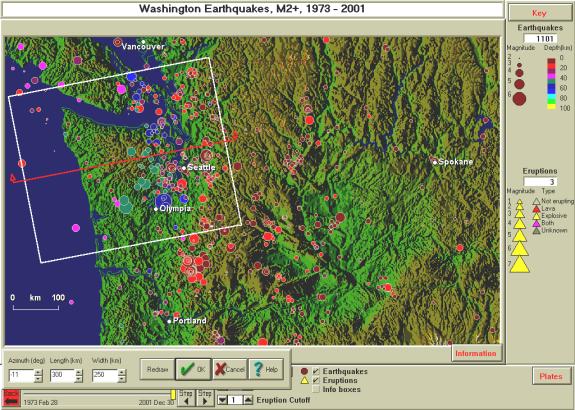
2. Select from the Map menu, Make Your Own Map. A dialog box will appear; click OK.

3. With the mouse, click and hold (drag) from the upper left hand corner of the area of interest to the lower right hand corner. A dialog box will appear; click Yes. The map will appear on the screen.

4. To get a better topographic background (shaded relief map) or to add topography if the screen (background) is blank, you can select an elevation file (etopo5 or topo30) if these files have been added to the TOPO folder within the SEISVOLE folder (see SeisVolE Teaching Module 1, “Downloading and Installing SeisVolE”), otherwise, go to 6.

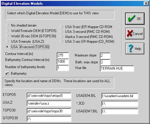
5. Select Shaded Terrain, Digital Elevation Models from the Map menu. A dialog box (below) will appear; in the upper left hand corner click on:

World 5-minute DEM (ETOPO5), if the area is outside the US, or,

USA 30-second DEM (TOPO30), if the area is in the conterminous US and you have added the topo30 elevation file.

In the lower left hand corner of the dialog box, be sure that the boxes to the right of ETOPO5 and TOPO30 look like the following:

ETOPO5 \seisvole\topo\etopo5.

TOPO30 \seisvole\topo\topo30.

Or, if you have installed SeisVolE in the D drive:

ETOPO5 d:\seisvole\topo\etopo5.

TOPO30 d:\seisvole\topo\topo30.

Click OK.

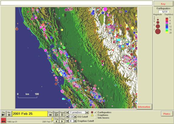
6. Select Redraw from the Map menu (move the cursor quickly away from the map area after selecting Redraw to avoid generating a blank area behind the mouse cursor position as the new map is drawn).

7. Adjust buttons at bottom of screen (magnitude cutoff, selecting earthquakes or volcanoes, etc.) if necessary.

8. Adjust menu items at top of screen (set dates, magnitude/depth scale, etc.) if necessary.

9. Add title, scale and city locations (select Annotations from the Map menu) if desired. City locations are added by selecting Add City from the Map, Annotations menu, and then clicking on the map near the location of a major city. Many city names and locations are stored in a SeisVolE file and the closest city to where you have moved the cursor and clicked will be added. If you add a city that you do not want, just use the Delete City option (from Map, Annotations) and click on the city that you wish to delete.

10. Click Repeat (at bottom of screen) to re-start earthquake sequence.

11. To save the view, select Save View As from the File menu. Choose a name (8 characters or less) that is different from the SeisVolE standard view names. After any changes have been made, use Save View As again (selecting the same name as you chose previously) to save the changes and avoid corrupting the standard view when exiting the program.

12. To save the image (for printing or exporting to another document), select Make Bitmap from the Options menu. You will be prompted for a file name. Save the Bitmap file in the SEISVOLE folder or other location. This file can be imported into an MS Word document or an image- or photo- processing program such as Adobe Photo Deluxe.

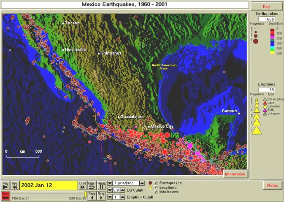
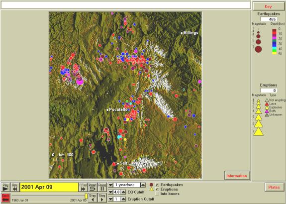
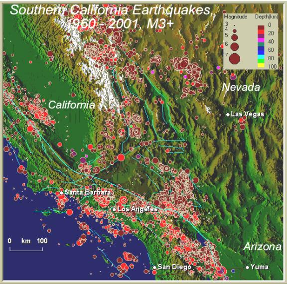
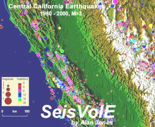
Examples, United States: Examples of several “Make Your Own Map” projects are given below. The maps that are created are intended to illustrate specific earthquake, volcanic activity or plate tectonic concept (in addition to illustrating the features of SeisVolE), or to focus on a specific area of interest. Several specific areas, such as California, Pacific Northwest, Hawaii, Japan, New Zealand, Taiwan, etc., are already included in the SeisVolE standard views. However, one can “zoom in” on a specific area of interest as illustrated by the “Make Your Own Map” example in Figure 11.1.

Figure 11.1. Earthquakes (1960 – 2001, M3+) in central California.

Additional earthquake catalogs are available (see Teaching Module 1) for selected areas. These catalogs provide additional data (smaller magnitude events or longer time period) that can be used in some of the SeisVolE standard views or for “Make Your Own Map” views. For example, in areas of fairly low earthquake activity, seismicity patterns are not very evident using the world.hy4 earthquake catalog (supplied with SeisVolE) that has data from 1960 and earthquakes of magnitude 4 and larger for the US (M3+ for California). Figure 11.2 shows northeastern United States (SeisVolE standard view) earthquakes of magnitude 2 and larger for the time period 1752 – 2001 using the eus.hy4 earthquake catalog. A total of 543 events are plotted and interesting clusters of epicenters are visible in several locations on this map. For comparison, the same view using the world.hy4 catalog (1960 – 2001, M4+) results in only 18 epicenters. The map in Figure 11.2 also illustrates the use of annotations (title, scale, and selected city locations) to make the map more useful. Using the “Make Your Own Map” option and the eus.hy4 earthquake catalog, one can create a map of any state or region of the central and eastern US that better illustrates the earthquake history of the selected area. Of course, all earthquake catalogs contain some data that are not precisely accurate, such as poorly determined locations or magnitudes, and are often incomplete, particularly for time periods more than a few decades ago because of inadequate seismograph coverage. These limitations are often visible when viewing the earthquake activity through time on the SeisVolE screen or from examining the data in the catalog.

Figure 11.2. Earthquakes (1752 – 2001, M2+) in the Northeastern United States. Earthquake data are from the eus.hy4 catalog (see Teaching Module 1). Title, scale and city names have been added using the Map, Annotations option in SeisVolE.

For the eus.hy4 catalog (and other catalogs that involve older data), earthquake locations for events that occurred before seismograph stations were available (these locations are called non-instrumental data) were determined from written reports (often newspaper accounts) of the ground shaking (called felt reports). Similarly, the magnitudes of these events were estimated from the intensity of shaking as described in the felt reports or from the area that was affected by the ground shaking for that event.

An effective teaching strategy using the “Make Your Own Map” option is to have students select a state, country or region to investigate using Seismic/Eruption. Several of the examples shown here are suitable for this approach. For example, selecting the state of Washington, one can create a detailed seismicity map with the Pacific Northwest earthquake catalog (pnw.hy4) as shown in Figure 11.3. Most of the earthquakes in Washington occur in the Puget Sound area just west of the Cascades Mountains. Some earthquakes, including some of the largest events in the Pacific Northwest historical record, are deeper (about 40 - 60 km; not the “deep earthquakes” that occur 300 – 700 km below the surface in subduction zones in the western Pacific and along the west coast of South America), for example, the Nisqually earthquake highlighted in Figure 11.3.

Figure 11.3 Earthquakes (1973 – 2001, M2+) in the state of Washington. Earthquake data for this area are contained in the pnw.hy4 catalog (see Teaching Module 1). The highlighted epicenter is the Nisqually earthquake (M6.8, February 28, 2001, near Olympia, Washington). The epicenter was highlighted using the Step tool (bottom of SeisVolE view screen). After the epicenter of interest has been found by “stepping backwards through the data”, clicking on the screen erases the information box but leaves the selected event highlighted.

To further examine the distribution of earthquakes beneath Washington, we can make a cross-section diagram (see Teaching Module 14). The location of the cross-section and area that is selected for the cross-section are shown in Figure 11.4. The resulting cross-section diagram is shown in Figure 11.5. In the cross-section, the hypocenters are projected onto a vertical “slice” through the Earth (along the red profile in Figure 11.4).

Figure 11.4. Earthquakes in Washington state and cross-section tool selection box (see Teaching Module 14).

Notice that in the cross-section view of earthquakes beneath western Washington (Figure 11.5), two distinct clusters of earthquakes are visible. Significant activity occurs in the crust beneath the Puget Sound lowlands area. The major population centers of Seattle, Tacoma, Everett and Olympia are affected by these events. Another concentration of earthquakes is deeper and appears to define the dipping slab of the Juan de Fuca plate that is being subducted (under-thrust) beneath the continental crust of western Washington. The three largest events in recent history (M6.9, April 13, 1949, 70 km depth; M6.7, April 29, 1965, 59 km depth; and M6.8, February 28, 2001, 52 km depth – the Nisqually earthquake highlighted in Figures 11.3 and 11.5) in Washington occurred in this slab beneath western Washington. The epicenters for these events are all close to Olympia, Washington. Because of the date ranges of the various earthquake catalogs, the pnw.hy4 catalog contains information on only one (Nisqually earthquake) of these events. The world.hy4 catalog contains information on the 1965 and 2001 earthquakes, and the sus.hy4 catalog (Significant US earthquakes; see Teaching Module 1) contains information on the 1949 and 1965 earthquakes.

Figure 11.5. Cross-section diagram corresponding to the profile (red line) and selection box (white rectangle) shown in Figure 11.4. West is to the left. The cross-section is formed by projecting the earthquake locations (foci, or hypocenters) that occur within the selection box onto a vertical plane (slice through the Earth) that intersects the Earth’s surface along the profile. The Nisqually earthquake hypocenter is highlighted in white. Additional labeling (white text, arrows and dashed lines) has been added in MS Word to help explain the pattern of hypocenters beneath western Washington. The horizontal scale on the cross-section is distance in kilometers from the profile location. The vertical scale is depth in kilometers below the surface.

An additional example of a state earthquake map created using the “Make Your Own Map” option in SeisVolE is illustrated in Figure 11.6. For the seismicity map of Utah, we have used the Intermountain Seismic Belt (ISB) earthquake catalog (isb.hy4, see Teaching Module 1) that includes earthquakes as small as magnitude 2. The ISB earthquake catalog contains data for the states of Idaho, Wyoming, Montana, Utah, Colorado, Arizona, and New Mexico. The Utah seismicity map indicates that most of the earthquakes in Utah are located along the Wasatch Front which forms the western boundary of the Rocky Mountains and the eastern boundary of the Basin and Range province in this area. The eastern boundary of the Basin and Range province, along the Wasatch Front, is a significant area of normal faulting (nearly east-west extension of the crust) in Utah. Notice that nearly all of the events are relatively shallow (<20 km depth).

Figure 11.6. Earthquakes (1973 – 2001, M2+) for the state of Utah. Earthquake data are from the isb.hy4 catalog (see Teaching Module 1). The shaded terrain map emphasizes the contrasting topography between the high Wasatch Mountains (just east of the cities of Logan, Salt Lake, Provo and Cedar City) and the north-south-trending ranges and valleys (called horsts and grabens) of the Basin and Range province to the west. The Great Salt Lake and Bonneville salt flats are visible to the west of Salt Lake City.

The state of Hawaii has an interesting and extensive earthquake and volcanic eruption history. Creating an earthquake map (Figure 11.7) of the Hawaiian Islands region of the Pacific Ocean indicates earthquake and volcanic activity but does not provide much detail. Most of the recent activity is associated with the “Big Island” of Hawaii and a SeisVolE standard view (Figure 11.8) is available to provide a closer and more complete picture of earthquake and volcanic activity in Hawaii. A special earthquake catalog and topographic data file are included in SeisVolE to produce this map. Displaying (“running”) the Hawaii view through time indicates that earthquake activity is very high and volcanic eruptions at Kilauea volcano are nearly continuous. Many of the earthquakes are located in the southeastern area of the island near the volcanic activity. An additional cluster of epicenters occurs off the south coast of the island. This activity is associated with a new, volcanically active seamount that may eventually become the next Hawaiian island. The 3000 m high (above the ocean floor) seamount is named Loihi. The top of Loihi is about 1000 m below the ocean surface.

Figure 11.7. Earthquakes (1960 – 2001, M5+) for the Hawaiian Islands area created using the “Make Your Own Map” option in SeisVolE. The world.hy4 (1960 – 2001, M5+) earthquake catalog and the etopo5 topographic file were used for this map.

Figure 11.8. Earthquakes (1960 – 1997, M3+) for the island of Hawaii. The view and earthquake catalog are from the Hawaii standard view in SeisVolE. A 3-second topographic data file was used to create the shaded terrain map.

Earthquakes in the central United States are not as common as in California or Alaska or other tectonically active areas of the world. However, earthquakes do occur in the central US, mostly related to the New Madrid seismic zone, and a seismograph network that has been operated in the area since 1974 provides a detailed view of seismicity patterns by plotting all events down to magnitude 1 (Figure 11.9). This map use the earthquake catalog nmeq.hy4, available for download from Teaching Module 1. “Make Your Own Map” views for states in this area should use the nmeq.hy4, eus.hy4 or sus.hy4 earthquake catalogs depending on the intended purpose.

“Make Your Own Map” views can be constructed with SeisVolE for any state or area of the United States. Special earthquake catalogs are available to provide smaller magnitude earthquake information or older, historic data. In addition to the California/Nevada (and other California “close-up” views), Pacific Northwest, New Madrid, Alaska, Hawaii, and Northeastern US views that are provided in SeisVolE, other states or regions of the US that are suggested for “Make Your Own Map” activities are: Washington, Oregon, Idaho, Nevada, Montana, Wyoming, Utah, Colorado, Arizona, New Mexico, Oklahoma, Kansas, Nebraska, Ohio, central Alaska, the Aleutian Islands of Alaska, southeast Alaska, and the northeastern US, southeastern US, and central US (New Madrid) regions or states within these regions. The eus.hy4, isb.hy4, nmeq.hy4, pnw.hy4, and sys.hy4 earthquake catalogs (see Teaching Module 1) are available for use with these states and regions as appropriate. Except for specific aftershock studies or other purposes where detailed data are required, the world.hy4 earthquake catalog supplied with SeisVolE provided excellent earthquake data for California, Nevada and Alaska because the catalog has been augmented to include earthquakes as small as 3 for California and Nevada, and because Alaska has so many M5+ events, the lack of smaller magnitude data does not significantly reduce the detail and impact of seismicity maps of Alaska. To view older historic data, the sus.hy4 or sww.hy4 (see Teaching Module 1) catalogs can be used. Finally, additional earthquake data for specific regions and for specific purposes can be extracted from the USGS earthquake catalog and imported into SeisVolE. For further information on this procedure, see Teaching Module 13.

Figure 11.9. Earthquakes (1974 – 2000, M1+) for the New Madrid area. Earthquake data are from the nmeq.hy4 catalog (see Teaching Module 1).

Examples, Other Regions Around the World: An excellent “Make Your Own Map” exploration or research project is to choose a country of the world and investigate the earthquake and volcanic history and related plate tectonics (of course, investigation of geology, geography, and culture could also be included to broaden the scope of the project). Starting with the SeisVolE North America view, a “Make Your Own Map” view of Mexico can be created (Figure 11.10).

Figure 11.10. Earthquakes (1960 – 2001, M5+) for Mexico. Earthquakes associated with divergent (red lines), transform (blue lines) and convergent (yellow lines) boundaries occur along the west coast of Mexico. Volcanic eruptions (39 during the period 1960 – 2001) are also common, about one per year, on average.

An additional example of a “Make Your Own Map” view for several countries is shown in Figure 11.11. Here we have focused on the northern Mediterranean region (starting from the SeisVolE Europe view) – primarily Italy and Greece. The tectonic setting of the Mediterranean is quite complicated, producing earthquakes and volcanoes, and mountain ranges, like the Alps, over much of the region. Of course you could “zoom in” further on any selected area. In fact, you can use the “Make Your Own Map” option on a map that has previously been created using the “Make Your Own Map” tool. You can also use the MS Word picture editing and draw tools (see Teaching Module 12) to crop the image (for example to remove the border area around the map on the SeisVolE screen if the legend information isn’t essential) and to add labeling such as in Figures 11.5 and 11.11.

Figure 11.11. Earthquakes (1960 – 2001, M5+) for the northern Mediterranean area including Italy and Greece.

Earthquakes in northwestern South America, including the countries of Colombia, Ecuador and Peru are shown in Figure 11.12. This is a very active area for both earthquakes and volcanic eruptions. Deep focus earthquakes are common in South America and indicate a variety of styles of subduction. Additional investigations of the depth distribution of earthquakes in South America (and other locations) can be conducted using the Cross-Section tool in SeisVolE (see Teaching Module 14).

Figure 11.12. Earthquakes (1960 – 2001, M5+) for northern South America.

Examples, Specific Geologic and Tectonic Features:

Figure 11.13. Earthquakes (1960 – 2001, M4+) for the Yellowstone and Snake River Plain area of the western United States.

Examples, Volcanoes:

Figure 11.14. Volcanoes of Mexico and Central America. Volcanoes are indicated by gray triangles. Erupting volcanoes (at the time shown on the slider at the lower left of the screen image; the view was paused at a time corresponding to December 11, 1966) are indicated by colored triangles and the volcano names are shown next to the triangles.

Figure 11.15. Volcanoes in the Kamchatka peninsula. Volcanoes are indicated by gray triangles. Erupting volcanoes (at the time shown on the slider at the lower left of the screen image; the view was paused at a time corresponding to January 31, 1982) are indicated by colored triangles and the volcano names are shown next to the triangles.

Figure 11.16. Volcanoes and earthquakes (1960 – 2001, M5+) in the Kurile Islands and Kamchatka peninsula area. Volcanoes are indicated by gray triangles. Screen image is from the SeisVolE Kuriles & Kamchatka standard view.

Examples, Mini-Posters:

Southern California earthquakes, 1960 – 2001; Prof. Lawrence W. Braile, Purdue University, April 2001. This map shows earthquake epicenters recorded by the US Geological Survey and by regional seismograph networks from January 1, 1960 to April 4, 2001. The map was produced using the SeisVolE computer program written by Prof. Alan Jones of the State University of New York, Binghamton (http://www.geol.binghamton.edu/faculty/jones). Epicenters are shown by colored dots. The dot size is proportional to magnitude of the earthquake. Depth of the earthquake is indicated by the color (see Key at upper right). Light blue lines are faults. The base map represents topography of the area using a shaded relief image. The map is made available by IRIS. IRIS is the Incorporated Research Institutions for Seismology, http://www.iris.edu.

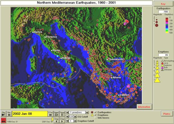
Figure 11.17. Earthquakes (1960 – 2001, M3+) for the southern California area. The image has been made into a “mini-poster” with the addition of annotations on the map and information about the data and map at the bottom of the image.

IDEAS:

Comparison of the number of earthquakes between states; the largest earthquake in each state; an active volcano in the state (where is it?), if not, where is the closest?; frequency/magnitude for map; compare number of earthquakes in regions of U.S. (NW vs. SE)

Assignment possibilities:

Choose your own state. Make a natural hazards brochure or poster. Also oral report and or written report.

Go to List of SeisVole Teaching Modules (in Introduction to SeisVolE Teaching…; Module 0)