EAS 557
Introduction to Seismology
Robert L. Nowack
Lecture 1
Overview and Terminology
Most of the Earth’s interior is not accessible to our direct observation. We can explore and map the surface, but drilling has only penetrated to about 13 kilometers in depth (by the Russians) and the average radius of the Earth is 6371 km. We are then forced to rely on indirect methods for information about a vast portion of the interior of the planet. The most powerful of these techniques is seismology: the study of elastic waves in the solid earth. Seismological methods allow us to map the Earth’s interior giving some idea of the distribution of physical properties with depth.
For example, the existence of a solid inner core for the Earth was inferred from seismic data. This was done in 1936 by a woman seismologist, Inge Lehmann, at the Danish Seismological Observatory. Similarly, discontinuities in seismic velocities at various depths in the Earth’s mantle, now considered the locations of geochemical phase changes, have been identified from the travel times of seismic waves. The depths of these phase changes place important constraints on the petrology and mineralogy of the Earth.
Seismic methods are also essential in exploring near surface structures for scientific and economic purposes. The oil industry spends hundreds of millions of dollars acquiring seismic data to guide exploration efforts.
Seismologists are also interested in the study of earthquakes, both as sources of elastic waves and as tectonic phenomena. It is possible to determine the nature of faulting in a distant earthquake by studying seismograms. This knowledge can be used to describe the motion of lithospheric plates where the earthquake occurred. Such studies provide a significant portion of our information about plate tectonics. Earthquakes are also studied because of their hazard on society. Our purpose in this course is to study seismic waves and sources in the solid Earth.
Seismic waves are a type of sound wave that travel in solids. For example, the speed of sound in air is .34 km/sec, ~ 760 miles/hr, ~ 1115 ft/sec and the speed of sound in water is about 1.5 km/s. Typical consolidated sedimentary rocks have compressional or “P” velocities from ~ 2.0-4.0 km/sec. Granite has compressional velocities near ~ 5.5 km/sec. Solids will also allow other types of motions, such as shear motions, which can’t be supported by air (or any fluid such as water).
Elastic waves have many similarities to light. For example, some basic principles of light can also be applied to elastic waves
a) We see color since light has different wavelengths.
b) The sky is blue because the atmosphere preferentially scatters certain wavelengths.
c) Light is bent when it travels into a medium of different velocity. Objects appear bent in water since light travels more slowly in water. This is called Snell’s law.
In the Earth, seismic velocity generally increases with depth. The waves bend further as they go deeper, and eventually bottom out and return to the surface. Seismic waves can also be reflected, as for example, by the Earth’s core. The amplitude of seismic reflections depends on the difference between the velocities and density on either side of the reflecting surface.
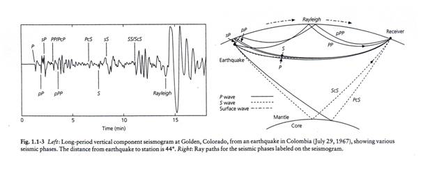
Figure 1 (from Stein and Wysession, 2003)
All these effects control what we see on a seismogram, which is just a record of the motion of the ground as a function of time resulting from some natural (earthquake) or artificial (explosion) source. The seismogram record in Figure 1 includes accurate timing and scaling information. The seismograph recording system must also be calibrated so we can convert the recording back to true motion of the ground.
We will see later that two basic types of elastic waves will propagate in the Earth (Figure 2).
1) “P”, compressional waves, correspond to particle motion along the wave path.
2) “S”, shear waves, correspond to particle motion perpendicular to the wave path.
In general, P waves travel faster than S waves.
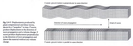
Figure 2 (from Stein and Wysession, 2003)
Almost immediately after the P in Figure 1 are the sP and pP arrivals. These are waves reflected off the Earth’s surface near the earthquake and then travel to the receiver. The sP phase travels up as a shear wave reflects and then travels as a P to the receiver. If we know the P and S velocities, we can use the times of these surface reflections to find out how deep the earthquake source was. A later arrival on Figure 1, labeled PcS, corresponds to a P wave down, reflected off the core “c”, and back up as an S.
In Figure 3, a seismogram from a
deep earthquake recorded at Kipappa (
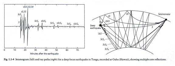
Figure 3 (from Stein and Wysession, 2003)
Much knowledge about the Earth’s interior have been derived from seismic data. Seismometers were also among the major experiments delivered to the lunar surface by the Apollo program.
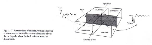
Figure 4 (from Stein and Wysession, 2003)
Seismograms can also tell a great
deal of information about earthquakes. For
example, for this South African earthquake in Figure 4, slip occurred on a
vertical fault plane with purely horizontal strike slip motion. The motion on the fault caused elastic waves
to radiate in all directions. In some
directions, the ground is pushed “away” from the source, while in other directions
“toward” the source. This situation
gives rise to different looking seismograms in different directions. This occurs in quadrants with respect to the
fault orientation. Mapping these
quadrants, one can estimate the orientation of faulting. This type of remote analysis of fault
orientation was used to prove the existence of transform faults in the mid-60’s
by Lynn Sykes at
Also, the routine location of earthquake epicenters can be used to map out major plate boundaries and deformation within plate (Figure 5). The study of seismic events as a function of location, fault geometry and magnitude is called seismotectonics.
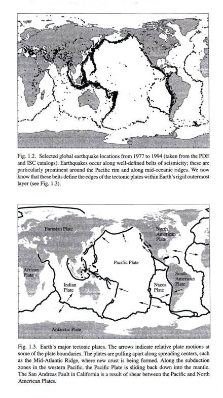
Figure 5 (from Shearer, 1999)
We are also
interested in studying large earthquakes because of the hazards they pose to
society. For example, the great 1906

Figure 6 (from Bolt, 1993)
Figure 7 shows a seismogram from
the 1906
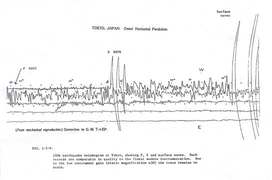
Figure 7
Direct
observation of the 1906
The
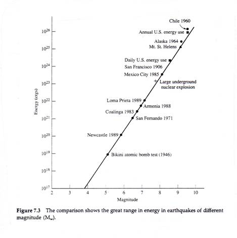
Figure 8 (from Bolt, 1993)
The estimation of earthquake hazards is important for the development of building codes and the assessment of property insurance rates. An example hazard map showing the degree of ground shaking expected at a 2% probability over a 50 year period is shown in Figure 9 (from the U.S. Geological Survey).
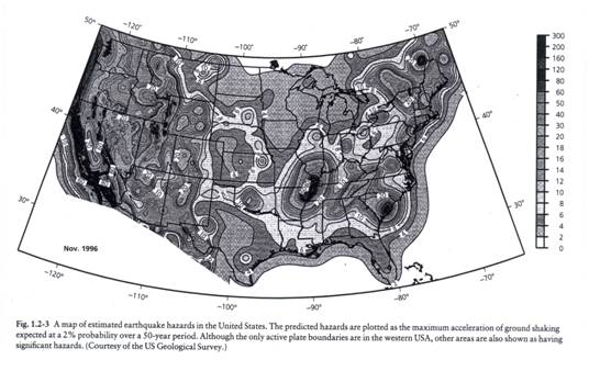
Figure 9
Another application of seismology is in the exploration of the Earth’s crust for minerals and hydrocarbons. Exploration geophysicists are interested in determining the structure at depth to search for petroleum (as well as mineral deposits). A typical seismic reflection profile is shown in Figures 10a and 10b. The analysis of such data is called seismic stratigraphy.
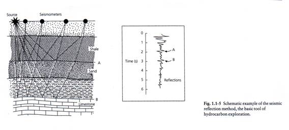
Figure 10a (from Stein and Wysession, 2003)
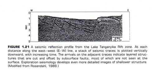
Figure 10b (from Stein and Wysession, 2003)
Seismic tomography methods are being applied for both crustal and whole Earth problems where seismic waves are used to “x-ray” the interior of the Earth.
Early investigations of Earth structure emphasized the estimation of the radially concentric part of the Earth structure (Figure 11).
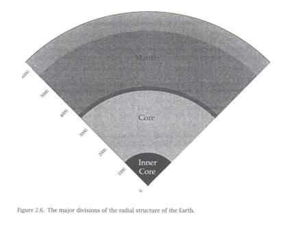
Figure 11 (from Kennett, 2001)
These are now used as reference models for the tomographic estimation of laterally varying Earth structure, such as those from subducting slabs (Figure 12).
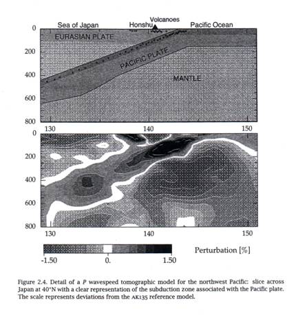
Figure 12 (from Kennett, 2001)
Complete tomographic inversions are now being performed for the estimation of complete Earth structure (Figure 13).
Figure 13 (from Shear, 1999)
The problems of Earth structure, earthquakes, and seismic exploration all involve basic concepts in elastic wave propagation. Our first priority will be to develop the necessary background in quantitative seismology starting with basic concepts.