EAS 557
Introduction to Seismology
Robert L. Nowack
Lecture 12
Seismic Sources Represented by Moment Tensors
We would like to model idealized seismic sources, for example, from earthquake sources and explosions. In order to model an earthquake source, assume a volume defined by two surfaces
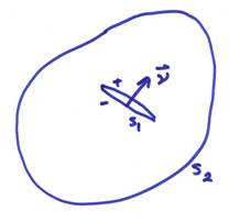
where the total surface is S = S1 + S2. Assume that either the displacement u or traction T(u) are zero on S2 and that ![]() = 0 in the volume. Thus, we will then only consider the surface
S1. For an earthquake source
then, there will be a displacement discontinuity on the plus side of S1
compared to the negative side of S1.
I’ll call the plus side of S1,
= 0 in the volume. Thus, we will then only consider the surface
S1. For an earthquake source
then, there will be a displacement discontinuity on the plus side of S1
compared to the negative side of S1.
I’ll call the plus side of S1, ![]() .
.
![]()
Inside S1 we will allow nonlinear effects, fracture, etc. All we require is that in the volume outside the bounding surface S1, things are continuous and linear. Assuming no body forces in the volume and continuous traction across S1, then the only term that results in nonzero displacements in the volume is from the displacement discontinuity across S1. This can be written

where ![]() is called the moment
tensor density mpg,
is called the moment
tensor density mpg, ![]() is the time
convolution, and
is the time
convolution, and ![]() is an element of the
fault surface
is an element of the
fault surface ![]() . See Aki and Richards
(1980) for a derivation of the representation theorem and this equation is their
Eqn. 3.2. Thus,
. See Aki and Richards
(1980) for a derivation of the representation theorem and this equation is their
Eqn. 3.2. Thus,
![]()
For a small compact source, then the resulting displacement will be
![]()
where ![]() is the moment tensor Mpq or in general
is the moment tensor Mpq or in general ![]() . Thus, for a small,
compact source
. Thus, for a small,
compact source
![]() (with sums on p and q)
(with sums on p and q)
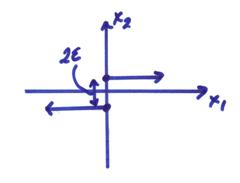
Now, what
is the meaning of  ? First, let’s write
this out for p = 1, q = 2 and
approximate the derivative by a finite difference. Then,
? First, let’s write
this out for p = 1, q = 2 and
approximate the derivative by a finite difference. Then,
![]()
The directed point forces giving rise to the Green’s
functions are in the plus and minus ![]() directions, but are
displaced in the
directions, but are
displaced in the ![]() direction by
direction by ![]() . This is called a force
couple.
. This is called a force
couple.
For ![]() , then the directed point forces giving rise to Green’s
functions are in the plus and minus
, then the directed point forces giving rise to Green’s
functions are in the plus and minus ![]() directions, but are also
displaced in
directions, but are also
displaced in ![]() by
by ![]() . This is called a force
dipole.
. This is called a force
dipole.
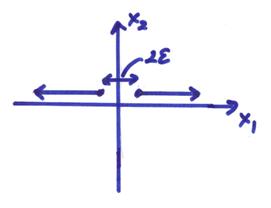
Thus, ![]() (moment tensor
density) is the strength of the (p,q) couple, where p is the force direction and q
is the offset direction of the couple.
Thus,
(moment tensor
density) is the strength of the (p,q) couple, where p is the force direction and q
is the offset direction of the couple.
Thus, ![]() has 9 strength
elements.
has 9 strength
elements.

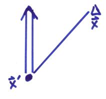
For a displacement discontinuity on a small crack, then
![]()
where ![]() is the moment tensor
density,
is the moment tensor
density, ![]() is the displacement
discontinuity or slip on the small crack,
is the displacement
discontinuity or slip on the small crack, ![]() is normal to the crack,
and cijpq are the elastic
constants.
is normal to the crack,
and cijpq are the elastic
constants.
For an isotropic
body ![]() , then
, then
![]()
For a shear slip or displacement discontinuity parallel to the face of the crack, the moment tensor density is
![]()
and the seismic moment is
![]()
Then,
![]()
where ![]() is the strength
parameter,
is the strength
parameter, ![]() is unit normal to
crack and
is unit normal to
crack and ![]() is the unit slip
vector direction along the crack.
is the unit slip
vector direction along the crack.
For a crack
in the ![]() plane,
plane, ![]() and for a slip
direction
and for a slip
direction ![]() , then
, then

where the 1 in M13 is the force direction and the 3 is the offset direction. For M31, these are reversed. Thus, a small crack can be modeled by two force couples with strengths M0.
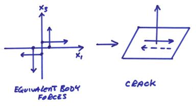
We can also write this in a 45o rotated coordinate system in terms of two dipole force couples.
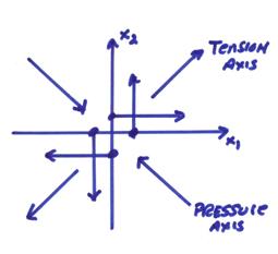
In general, a double couple source must have the trace of the moment tensor matrix equal to zero. Note that each dipole would cause a net rotation. The other dipole in the force system is imposed by the continuum so that there is no net rotation in the solid by the fracture. So, for a shear crack source, couples come in pairs. This is called a double couple model for an earthquake source.
What we’ve really done is replace a complicated crack model with an equivalent set of forces such that
![]()
where ![]() for an arbitrarily complicated
(but linear) medium is the Green’s function.
The moment tensor for a small earthquake crack is
for an arbitrarily complicated
(but linear) medium is the Green’s function.
The moment tensor for a small earthquake crack is
![]()
Note that if we replace ![]() by the
by the ![]() direction, we get the
same result. Thus, there is an ambiguity
between the crack normal and the slip direction which must be resolved with
other geologic input. The value M0
is the strength parameter and is called the scalar seismic moment. It has the units of force times a length.
direction, we get the
same result. Thus, there is an ambiguity
between the crack normal and the slip direction which must be resolved with
other geologic input. The value M0
is the strength parameter and is called the scalar seismic moment. It has the units of force times a length.
In seismology, we often use units of dyne-cm (or Newton-meters in SI units). From the above formulas for an earthquake model
![]() scalar seismic moment
scalar seismic moment
where ![]() is the fault area,
is the fault area, ![]() is shear modulus
(about 3 x 10¹¹ dyne/cm2 for crustal rocks), and
is shear modulus
(about 3 x 10¹¹ dyne/cm2 for crustal rocks), and ![]() is average slip on the
crack.
is average slip on the
crack.
The range of values for the scalar seismic moment are

The moment magnitude can be derived from the scalar seismic moment as
![]()
for M0 in dyne-cm (see Stein and Wysession, p. 266).
For a volume source, like an explosion, the moment tensor would have a form as
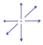
and can be modeled by three in-line force dipoles along the coordinate directions. Thus,

where ![]() , in this case, is the strength parameter for the explosive
source.
, in this case, is the strength parameter for the explosive
source.
In a homogeneous media, the far field Green’s function can be written from the last lecture as
 far field P
 far field S
where ![]() is the unit vector
from the source
is the unit vector
from the source ![]() to the receiver
to the receiver ![]() .
.
where
![]()
and
![]()
For the far field P wave ![]() , then
, then

Dropping all terms which decay faster than ![]() , then
, then
![]()
Assuming the displacement fault slip is the same everywhere for a very small fault, then
![]()
where si is the slip vector. The far field wavefield is then
 far field P wave
 far field S wave
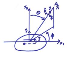
Referring to the figure above, the far field radiation pattern terms can be written
![]()
![]()
The following comments can be made about the far field radiation from a shear crack in a homogeneous medium:
1) The far field P wave particle motion is parallel to the direction of propagation.
2) The far field S wave particle motion is perpendicular to the direction of propagation.
3) The far field P and S waves decay in
amplitude as ![]() .
.
4) The S wave amplitude is ![]() times larger then the
P-wave amplitude. For a Poisson solid
with
times larger then the
P-wave amplitude. For a Poisson solid
with ![]() , then the S wave amplitude is about 5 times larger than the
P-wave amplitude.
, then the S wave amplitude is about 5 times larger than the
P-wave amplitude.
5) AFP – The directional radiation
pattern for P-waves in the ![]() plane is
plane is
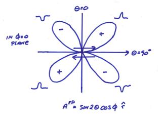
Fault plane solutions use just the
sign bit information of many remotely recorded P waveforms to infer the fault
strike and slip directions ![]() and
and ![]() and, thus, the
orientation of faulting. We will
investigate this further later in the class.
and, thus, the
orientation of faulting. We will
investigate this further later in the class.
6) AFS – The directional radiation
pattern for S-waves in the ![]() plane is
plane is
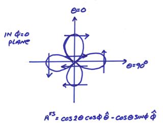
7) Note that we have neglected near field terms
with amplitudes ![]() which will be small in
the far field where
which will be small in
the far field where ![]() dominates.
dominates.
8) The far field displacement wavefield ![]() is proportional to
time derivative of slip time function on the fault
is proportional to
time derivative of slip time function on the fault ![]() .
.
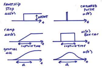
Thus, the measurement of the
seismic pulse width of the radiated P- or S-wave pulse gives information about
the time of fault slip at a point on the fault.
This is also called the rise time.
In addition, a finite fault will have a rupture time related to the
length of faulting divided by the rupture velocity, which is often assumed to
be .7![]() . The total rupture
time will be related to the rise time and the rupture time on the fault. The measurement of the far field P-wave or
S-wave pulse spectrum
. The total rupture
time will be related to the rise time and the rupture time on the fault. The measurement of the far field P-wave or
S-wave pulse spectrum ![]() will also provide
information on the duration of rupture.
will also provide
information on the duration of rupture.
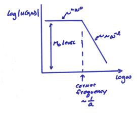
A simplified model of the radiated energy from a small earthquake source is shown below where low frequency level is proportional to M0 and the corner frequency is proportional to one over the total time of rupturewhere the total rupture time is related to the fault size.
For an explosion in the far field, then
![]()
where,
1) For an explosion, the S wave “theoretically doesn’t exist”. But, real explosions do generate some S-wave energy.
2) The displacement is a spherically symmetric outward pulse.
3) A step function pressure pulse at the source gives rise to a radiated delta function in the far field.
Finally, in a slowly varying media where ray theory can be used, then for a P wave
![]()
where ![]() is used instead of
is used instead of ![]() for the heterogeneous
case, T is the geometric travel time, J is the geometric spreading and A is related
to the source strength and additional reflection/transmission coefficients.
for the heterogeneous
case, T is the geometric travel time, J is the geometric spreading and A is related
to the source strength and additional reflection/transmission coefficients.