EAS 557
Introduction to Seismology
Robert L. Nowack
Lecture 13A
I. Reflection and Transmission of Waves at Boundaries
There are several different kinds of boundary conditions that we will consider.
a) Welded boundaries
This
boundary condition requires continuous particle displacements and
tractions. The normal to the boundary at
a given point is noted by ![]() pointing from the
negative side to the positive side of the boundary.
pointing from the
negative side to the positive side of the boundary.
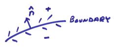
1) Displacements are continuous. This can be written
![]()
where ![]() and
and ![]() are on the plus and
minus side of the boundary.
are on the plus and
minus side of the boundary.
2) Tractions on the surface are continuous. This requires
![]()
b) Solid-fluid boundaries (i.e., the ocean bottom or the core-mantle boundary)
This is the same as for the welded case, except now lateral slip along the boundary can occur. Thus, only the component of displacement normal to the boundary will be continuous. But, tractions will still be continuous. Thus,
![]()
and
![]()
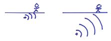
c) Free surface (i.e., the Earth’s surface)
An example of a free surface is the surface of the Earth. (In fact, this could be modeled as a fluid-solid boundary except that the properties of the air are so much different than the solid that it is sometimes modeled as a free surface.) Thus, the boundary conditions are zero tractions on the boundary.
![]()
There is no restriction on displacements.
These general boundary conditions must be satisfied at all discontinuities in the medium.
No matter what computer program one uses (finite differences, finite elements, etc.), one must use these boundary conditions. A welded boundary has six total boundary conditions, a fluid solid boundary has four total boundary conditions and a free surface has three boundary conditions.
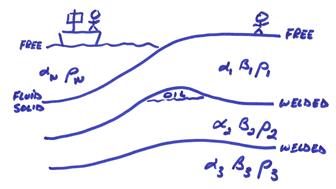
Examples in the Earth of different boundaries are:
The Earth’s surface (solid, fluid) – free surface
Ocean-seafloor – fluid-solid
Basement sediments – wielded
Depositional discontinuities – welded
Conrad discontinuity in continental crust – welded
Moho discontinuity between crust and mantle – welded
“410” and “660” upper mantle discontinuities – welded
Core mantle boundary – fluid-solid
Outercore-innercore – fluid-solid
Earlier, we found the wavefields for a point force, a double couple shear source, and an explosion source in a whole space.
For the source sufficiently far away from a boundary, the wavefront will be effectively planar. Thus, as an approximation, planar waves can be assumed for a very distant source.
Earlier, we found that a plane wave could be written in complex form as
![]()
where it was found that ![]() is the wavenumber
vector and points in the direction of propagation. The magnitude of
is the wavenumber
vector and points in the direction of propagation. The magnitude of ![]() where c is the wave velocity.
where c is the wave velocity.
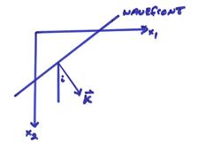
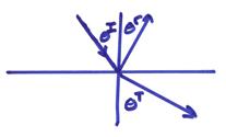
In 2D, ![]() . From the diagram
above,
. From the diagram
above,
![]()
Sometimes we will also use the slowness vector
![]()
where c is the wave speed.
Both P-waves and S-waves can propagate in the far fiield
1) P
waves. The speed is ![]() and the particle
motion
and the particle
motion ![]() is parallel to
is parallel to ![]() .
.
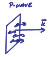
Thus, for a ![]() vector in the x1 direction,
vector in the x1 direction, ![]() and
and
2) S
waves. The speed is ![]() and the particle
motion
and the particle
motion ![]() is perpendicular to
is perpendicular to ![]() .
.
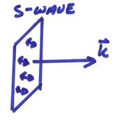
Thus, for a ![]() vector in the x1 direction,
vector in the x1 direction, ![]() and
and
The flux rate of energy transmission in a plane wave (the
amount of energy transmitted per unit time across unit area normal to the
direction of propagation) is proportional to ![]() for P waves and
for P waves and ![]() for S waves. This is a local property depending on
for S waves. This is a local property depending on
a) Material parameters
b) Local planar nature of wavefront
c) E is related squared amplitude through ![]() .
.
d) Depends on ![]() , which is the seismic impedance, where c is the particular wave speed.
This is also related to the ratio of stress to particle velocity.
, which is the seismic impedance, where c is the particular wave speed.
This is also related to the ratio of stress to particle velocity.
The energy
flux across a tilted plane is proporational to ![]() , where c is the
wave speed and i is the angle of the
tilt. We will later find that reflection
coefficients will depend on mis-matches in the seismic impedance across layer
boundaries.
, where c is the
wave speed and i is the angle of the
tilt. We will later find that reflection
coefficients will depend on mis-matches in the seismic impedance across layer
boundaries.
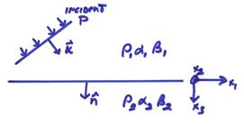
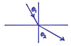
We will now
assume a plane wave incident on a plane boundary. In order to simplify the problem, a local
coordinate system will be centered at the boundary with the (x1,x3) plane determined by the incident ![]() vector and the normal
to the boundary
vector and the normal
to the boundary ![]() . This is called the
plane of incidence. An incident P-wave
is first shown.
. This is called the
plane of incidence. An incident P-wave
is first shown.
The orientation of the interface will “polarize” the S waves into “SV” waves with particle motions in the plane of the incidence “SH” waves with particle motions perpendicular to the plane of incidence.
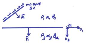
Positive P, SV, and SH will be chosen with regards to (x1,x2,x3) local coordinates of the interface for the incident, transmitted, and reflected waves. Note that other sign conventions can be used, but if one knows what they are, one can change them as required.
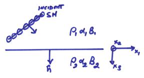
For an incident “SH” wave, the particle motions of the incident wave and all scattered waves are perpendicular to the plane of incidence.
In order to solve for the reflected and transmitted wave, we first apply the boundary conditions for a welded interface.
a) Apply continuity of displacement at x3 = 0. Then,
![]()
where we will assume the incident wave to
be an SH wave, then ![]() or
or
where
with
![]()
![]()
Also,
![]()
![]()
for the reflected and transmitted waves.
b) Apply continuity of tractions at x3 = 0. In terms of the stress matrix, this can be written
![]() where
where 
and the stress matrix for isotropic media can be written
![]()
The tractions
are then ![]() . For
. For 
![]()
then,
![]() ,
, ![]()
![]()
For a plane wave of the form
then,
![]() ,
, ![]() ,
, ![]()
Now,
![]()
![]()
![]()
![]()
then, for continuity of traction
![]()
Note for the incident “SH” case, there is no coupling of A2 with A1, A3 for continuity of displacements or tractions. Then,
and
For continuity of displacement and traction, then
![]()
![]()
where both are evaluated at x3=0.
First, these equations will only be true if the phase is the same for all terms. This will occur if
![]()
where
Thus,  . This is commonly
called Snell’s law. In French, this is
sometimes called Descartes law
. This is commonly
called Snell’s law. In French, this is
sometimes called Descartes law
Another way of saying this is that the horizontal component of the wavenumber is unimpeded by a horizontal interface.
In
seismology, the slowness vector is also used where ![]() . Thus,
. Thus,
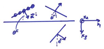
Snell’s law also states that the horizontal component of the slowness vector travels without being impeded by a horizontal interface. Thus, upon reflection, assuming no phase conversion from P to S (as there would be for the in-plane P-SV case), then
1) The first simple law of geometric optics is
or this says that the angle of reflection
is equal to the angle of incidence, regardless of the material properties
across the boundary. This is also called
2) For transmission, then
Thus, for ![]() ,
, ![]() .
.
Comments
a) The phase relations don’t depend on density, only on velocity. Thus, phase information or travel times cannot give a complete picture of the Earth’s interior.
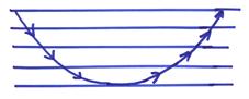
b) For an earth with increasing velocity with
depth, then downgoing “rays” represented by the wavenumber vector ![]() will flatten with
depth and then turn back up to the surface.
will flatten with
depth and then turn back up to the surface.
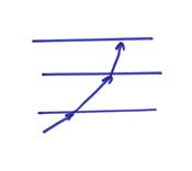
c) Upward traveling “rays” will steepen for lower velocity layers
d) In horizontally layered structures, the
horizontal slowness, ![]() , does not change along the path, where c is the wave speed. This is
given a special name and symbol
, does not change along the path, where c is the wave speed. This is
given a special name and symbol
![]() = ray parameter
= ray parameter
since in a vertically varying medium, p uniquely identifies the “ray” going through the structure.