EAS 557
Introduction to Seismology
Robert L. Nowack
Lecture 8
Constitutive Relations
We have so
far not specified the relationship between displacement and forces in the
continuum. The relationship between ![]() (strain) and
(strain) and ![]() (stress) is termed a
constitutive relation. Constitutive
relations can be {linear/nonlinear}, {time dependent/time independent},
{reversible/nonreversible}.
(stress) is termed a
constitutive relation. Constitutive
relations can be {linear/nonlinear}, {time dependent/time independent},
{reversible/nonreversible}.
In general terms, the behavior of a solid under stress can be roughly characterized by a stress-strain relation having some, or all, of the following features
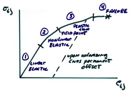
1) linear elastic (i.e., Hookean)
![]() = linear function of eij
= linear function of eij
reversible process (recoverable strain energy)
slope of ![]() gives elastic
constants
gives elastic
constants
2) nonlinear elastic
![]() is a nonlinear
function of
is a nonlinear
function of ![]()
reversible – strain energy recoverable
characteristic of soils
3) yield region ~ beyond the yield point or elastic limit,
ductile region, plastic flow
energy is dissipated
unloading leaves permanent offset
- grain sliding and rotation
- microfracturing
This could be accompanied by dilatancy which is an increase in specific volume resulting in a decrease of seismic velocities. In the 1970’s, this was thought to have great potential for predicting earthquakes.
strain hardening
4) failure ~ region beyond ultimate strength of the material
proceeds catastrophically to failure
The condition can be very unstable ranging over a cascade of distance scales
Viscoelasticity – This refers to time dependent constitutive relations
The Earth primarily acts at short time scales as an elastic body, but at long times, it can flow or creep without obvious faulting. Strain rate is then proportional to applied stress.
There are a number of simple models for viscoelastic materials.
Viscoelastic Rheological
Models
1) Elastic Material
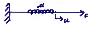
![]()
where F is a force, ![]() is the elastic
constant (or spring constant), and u
is the displacement. For a continuum,
this would be
is the elastic
constant (or spring constant), and u
is the displacement. For a continuum,
this would be
![]()
2) Viscous Material
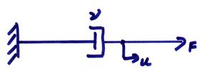
where for example this could represent the pulling of a plate through a fluid in a dashpot. Then,
![]()
where F is the applied force, ![]() = viscosity, and
= viscosity, and ![]() is the particle
velocity. For a continuum, this would be
is the particle
velocity. For a continuum, this would be
![]()
For this case, a constant stress results in a constant strain rate.
Units of viscosity are in poise where 1 poise = 1 dyne -s/cm2. In SI units, viscosity is in Pascal-sec where 1 poise = 0.1 Pa-s.
3) Maxwell solid
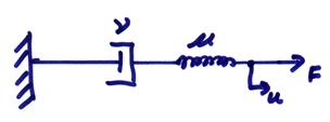
where this shows a spring and dashpot in series. Then,
![]()
The material is elastic at short times and viscous at long times
4) Voight (Kelvin solid)
In this model, the spring and dashpot are in parallel.
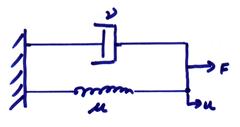
Then,
![]()
In the frequency domain, this can be written as
![]()
where ![]() is a complex elastic modulus,
and
is a complex elastic modulus,
and ![]() and
and ![]() are the Fourier
transforms of
are the Fourier
transforms of ![]() and
and ![]() .
.
In elastic wave problems, slight dissipation can be modeled using complex elastic constants and the same equation as for the elastic case can be used. This is called the correspondence principle.
In the Earth, observations indicating a dissipation loss mechanism, include
Attenuation of seismic waves as measured by a “Q” value
Damping of the Earth’s
Nonhydrostatic figure of the Earth
Uplift and subsidence of land masses
(Fennoscandia) (
For seismic wave propagation, linear elasticity works to an excellent degree away from the source region. Seismic attenuation (not including scattering) can also be included using a Q value related to the imaginary part of the elastic constant. Below, we will focus on linear elasticity with real elastic constants.
We consider, in the seismic wave propagation context, linear elasticity and infinitesimal strain. Assume a Hooke’s Law relation
![]()
where ![]() are the elastic
constants which has 34 or 81 components (each index going from 1 to
3).
are the elastic
constants which has 34 or 81 components (each index going from 1 to
3).
We now
apply various constraints on ![]() to reduce the number
of elastic constants:
to reduce the number
of elastic constants:
1) From
the symmetry of ![]() and
and ![]()
![]()
then
![]()
This reduces the number of independent elastic constants from 81 to 36.
2) From existence of strain energy function, where W = internal energy per unit volume, then by energy considerations of an adiabatic reversible process
![]()
From linear elasticity, ![]() , and W can be written as a quadratic and homogeneous
function of
, and W can be written as a quadratic and homogeneous
function of ![]()
![]()
![]() by symmetry
by symmetry
Thus,
![]()
The number of independent elastic constants then reduces from 36 components to 21.
In Love’s notation
or
![]()
where L = 1,6 and M = 1,6. The relation between CLM and cijkl is given by
|
L |
(ij) |
|
1 |
11 |
|
2 |
22 |
|
3 |
33 |
|
4 |
23 or 32 |
|
5 |
13 or 31 |
|
6 |
12 or 21 |
For example,
C66 = c1212 = c2112 = c1221
For various crystal symmetries, the 21 independent elastic constants can be progressively reduced in number, ultimately reaching 2 constants for a perfectly isotropic material.
Ex) A triclinic crystalline substance has 21 elastic constants
Ex) A monoclinic crystal has symmetry with respect to one plane and has 13 independent elastic constants
Ex) Orthorhombic symmetry has symmetry with respect to three planes and has 9 independent elastic constants
Ex) Hexagonal symmetry has 5 independent elastic constants
For example, “transverse isotropy is common in seismology and has symmetry in a plane perpendicular to the z axis. This is common in seismology related to stacks of thin layers with a vertical axis of symmetry. In general, hexagonal symmetry can have an arbitrary axis of symmetry and can result from crystal symmetry, a stack of thin layers in a sedimentary rock, or a crack network in a rock.
The Love matrix for hexagonal symmetry is
An excellent survey of wave propagation in general anisotropic materials is given by Auld (1990). Applications of seismic anisotropy in the Earth are given by Babuska and Cara (1991).
Proceeding in this way, we come to the case where the constants are invariant to an arbitrary rotation of the coordinate axes. This is called isotropy. Although no crystal has this symmetry, it is the most common one used in elasticity and seismology. It is appropriate for fine-grained materials with grains with random orientations.
The Love matrix for an isotropic material is
The Lamé constants for an isotropic material are ![]() which is called the
shear modulus,
which is called the
shear modulus, ![]() and
and ![]() . Then,
. Then,
In full index notation, the isotropic elastic constants can be written as
![]()
where
![]()
Expressing the stress-strain
relation for a linear elastic solid as ![]() , then for an isotropic material
, then for an isotropic material
![]()
For each component, this can be written as
In addition to ![]() and
and ![]() , other isotropic elastic constants are sometimes easier to
measure in the lab.
, other isotropic elastic constants are sometimes easier to
measure in the lab.
1) Young’s Modulus
Consider a bar under uniaxial compression (or tension) ![]() , then
, then
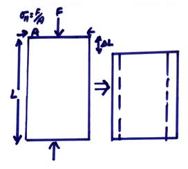
For this case,
![]()
where E is called Young’s Modulus and is measured as the ratio of uniaxial stress to strain.
2) Poisson’s ratio = ![]()
Poisson’s ratio is the ratio of contraction in the direction of applied stress to the expansion in directions perpendicular to the applied stress. Thus,
![]() (
(![]() is
not viscosity here!)
is
not viscosity here!)
where L2 is a direction perpendicular to the direction of applied stress. Then,
![]()
The two constants ![]() can be used to
describe the isotropic elastic properties in a similar manner as
can be used to
describe the isotropic elastic properties in a similar manner as ![]() and are easier to
measure.
and are easier to
measure.
Now, we want to relate ![]() to
to ![]() . For uniaxial
compression,
. For uniaxial
compression,
![]()
![]()
![]()
Then,
a) ![]()
b) ![]()
From these, we can find
relations between ![]() and
and ![]() as
as
![]()


Now consider a bar under hydrostatic stress
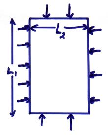
where,
![]()
(recall pressure is positive in compression).
Now, find the forces in the different coordinate directions and relate to the strain in the x1 direction.
a) forces in x1 
b) forces in x2 
c) forces in x3 
where ![]() is the Poisson’s ratio
and E is Young’s Modulus. Then, the
total change length in the x1
direction from all applied stresses is
is the Poisson’s ratio
and E is Young’s Modulus. Then, the
total change length in the x1
direction from all applied stresses is

The change of volume can then be written as
![]()
Thus,
![]()
K is called the bulk modulus relating an applied hydrostatic pressure to a change of volume.
Under an applied shear stress, say ![]() , with all other stresses being zero, then
, with all other stresses being zero, then
![]()
Thus, shear modulus ![]() is related to the
ratio of shear stress to shear strain.
Note, with our definitions of stress, there is also a factor of 2.
is related to the
ratio of shear stress to shear strain.
Note, with our definitions of stress, there is also a factor of 2.
We can relate K to ![]() as
as ![]() . Thus, we could also
use
. Thus, we could also
use ![]() as the independent elastic
parameters for an isotropic material.
as the independent elastic
parameters for an isotropic material.
The
coefficients ![]() and
and ![]() are related to the
more commonly measured elastic coefficients by
are related to the
more commonly measured elastic coefficients by
![]() = G = shear modulus
= G = shear modulus
E
= Young’s modulus = ![]()
![]() = Poisson’s ratio =
= Poisson’s ratio = ![]()
K
= Bulk modulus = ![]()
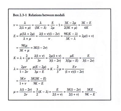
A complete set of relations for an isotropic medium is given in the box below from Stein and Wysession (2003).
Poisson’s
ratio is a very important diagnostic property of an isotropic elastic
material. It can vary from -1 to +.5. For a perfectly rigid material, ![]() = 0. For an incompressible fluid,
= 0. For an incompressible fluid, ![]() = .5 and
= .5 and ![]() .
.
When under uniaxial compression, a material with a Poisson’s ratio of zero won’t come out on the sides. An example of this type of material is cork which is used as a bottle stopper. A material with a negative Poisson’s ratio would come in on the sides under uniaxial compression. But, it is important to remember that Poisson’s ratio is an isotropic and not anisotropic concept.
The solid part of the Earth (coast
to mantle) has a Poisson’s ratio that varies between .25 to .30. For a Poisson solid, we choose ![]() and for this case
and for this case ![]() . This relation is
assumed in a great number of seismic studies of the solid parts of the Earth. In the Earth’s liquid outer core,
. This relation is
assumed in a great number of seismic studies of the solid parts of the Earth. In the Earth’s liquid outer core, ![]() . In the inner core,
which is in a solid state,
. In the inner core,
which is in a solid state, ![]() ~ 0.40-0.45. That is, the inner core can support shear,
but is quite different from the mantle material.
~ 0.40-0.45. That is, the inner core can support shear,
but is quite different from the mantle material.