EAS 657
Geophysical Inverse Theory
Robert L. Nowack
Lecture 4
Optimization in a Hilbert Space
With an inner product, I.P., defined, we can perform a direct sum decomposition of V, thus

V = V1 + V2
Note in a direction sum decomposition, V1 and V2 are orthogonal subspaces, but don’t include all vectors in V.
Now for every I.P., we can find an orthonormal bases via Gram Schmidt. The converse is also true. For any basis for V {v1…vn} we can find some inner product for which these vectors are orthonormal. (This can be used later to show that optimality depends on the particular inner product and error norm chosen!)
Now, the problem for given any vector v and subspace V1 in V,

find a vector in V1 which is the “best approximation” to v, i.e., find a vector v1 in V1 which is “closest” to v in some sense. Alternatively, given an error vector e = v – v1, we want to minimize e.
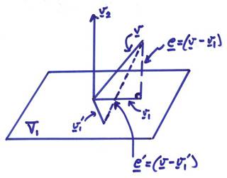
The projection theorem states that given a
vector v in V and a subspace V1, there exists a unique
vector ![]() such that | e | = || v – v1
|| is minimized. In addition, the
vector e is orthogonal to the
subspace V1.
such that | e | = || v – v1
|| is minimized. In addition, the
vector e is orthogonal to the
subspace V1.
1) Decompose V into ![]() where
where ![]() by a direct sum
decomposition of an orthogonal basis. Let,
the vector v = v1 + v2 where
by a direct sum
decomposition of an orthogonal basis. Let,
the vector v = v1 + v2 where ![]() .
.
An arbitrary error vector can be written, where ![]() as
as
![]()
Now,
![]()
The error is minimized if we let ![]() . Then,
. Then, ![]() where the error vector
e is perpendicular to all
vectors in V1.
where the error vector
e is perpendicular to all
vectors in V1.
Many optimization problems in a Hilbert Space are based on this idea!
Application of
Projections
Ex) Let V
= R2 be spanned by ![]() and
and ![]() .
.
Gram Schmidt can be used to find the projection of v2 onto v1. First,
![]()
The first vector is already normalized. The projection of v2 onto v1 is
![]()
Now,
![]()
or
![]()
This is also normalized, thus ![]() .
.
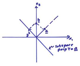
Ex) Find the projection of  onto the subspace
defined by the equation aTx
= 0 (defining an R2
subspace perpendicular to the vector a)
where
onto the subspace
defined by the equation aTx
= 0 (defining an R2
subspace perpendicular to the vector a)
where  and V = R3.
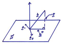
Let the subspace spanned by a be called Sperp and the plane perpendicular to a be called S. Then,
S + Sperp = V = R3
Any vector can then be uniquely projected onto S and onto Sperp. In this
case, it is easiest to first project onto ![]() . Let
. Let
 (the normalized
version of a)
(the normalized
version of a)
Now,
![]()
then,

and

Thus the vector bS in S that “best approximates” ![]() is its projection onto
S.
is its projection onto
S.
We can always represent an arbitrary vector x in terms of a basis in V. Thus,
![]()
If we have constructed an orthonormal basis, ![]() , then we can write
, then we can write
![]()
Ex) Let v(t) be a periodic signal space V with period T such that
![]()
Now let,
![]()
where v1(t) is also a periodic signal with period T in a subspace V1 spanned by the first 2M + 1 Fourier coefficients with M < N. Then the best approximation of a signal v(t) in the subspace V1 is just the truncated series. However, a smoother signal could be obtained by tapering the truncation window, but this would require a modified inner product.
Ex) In R3
with a standard inner product, what is the best approximation to the vector  in the x1 – x2 plane? It is
just the vector
in the x1 – x2 plane? It is
just the vector  .
.
Ex) What is the best approximation to the
vector in the subspace V1 defined by 8x + 5y
+ 4z = 0? The projection theorem states that we must
decompose v into ![]() and
and ![]() , then
, then
v = v1 + v2
where
![]()
Let a subspace
S be spanned by the columns of a
matrix A (M x N) in RM. For the case above, find two independent
vectors in V1 perpendicular to ![]() and put as columns of
A. Now project a vector b onto the subspace S spanned by the column vectors a1, a2, … aN. Then,
and put as columns of
A. Now project a vector b onto the subspace S spanned by the column vectors a1, a2, … aN. Then,
bP = x1a1
+ x2a2 … xNaN or,
bP = Ax = [a1, a2,
… aN] ![]()
Now, the error vector e will be perpendicular to all vectors in S. Then for e = b – Ax
 AT(b – Ax) = 0
This gives
ATb = ATA x
and
x = (ATA)-1 ATb
(Note: for independent columns of A, (ATA) is invertible, i.e. if the columns of A, a1, a2, … aN form a basis for S.
Then,
bP = Ax = A(ATA)-1AT b
This is the general case of projecting a vector b onto a subspace S with a basis specified by the columns of a matrix A.
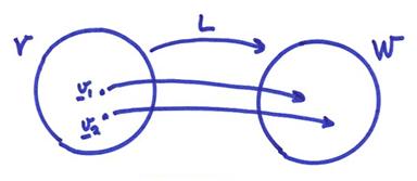
Linear Transformations
Between Finite Dimensional Vector Spaces
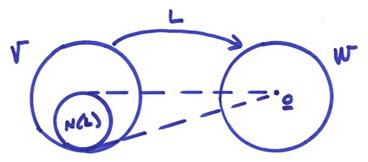
Let L map a vector ![]() to a vector
to a vector ![]()

A linear transformation satisfies
1) L(v1 + v2) = L(v1) + L(v2)
2) L(av) = aL(v)
The second part can be remembered as: if a system is linear, then “if you double the input, you double the output”.
A linear transformation is “onto” if for any ![]() , there is a vector
, there is a vector ![]() such that L(v)
= w
such that L(v)
= w
The “range” of a linear transformation is the subspace corresponding to L(v). This is referred to as R(L) (for an “onto” transformation R(L) equals all of W).

A linear transformation is “one-to-one” if for any ![]() , there is a unique v
such that L(v) = w.
, there is a unique v
such that L(v) = w.
A linear transformation is “invertible” if
1) it is one-to-one (invertible on its range)
2) onto
The “null space” of a linear transformation, N(L) is the subspace of V defined by the vectors vi, such that L(vi) = 0.
Dim{N(L)} =
0 if and only if the transformation is one-to-one. To show this, assume L is not one-to-one. Then there exists vectors v1 and v2, such that L(v1)
= L(v2) = w. Then, L(v1) – L(v2)
= L(v1 – v2)
= 0. Then, ![]() , but N(L) = {0}, so (v1
– v2) = 0 and v1 = v2.
, but N(L) = {0}, so (v1
– v2) = 0 and v1 = v2.
Eigenvectors and
Eigenvalues
These are defined
for L:V ![]() V. If
V. If ![]() , then
, then ![]() is called an
eigenvalue of L and v is the
corresponding eigenvector. (More on this
will be given with respect to matrices later).
is called an
eigenvalue of L and v is the
corresponding eigenvector. (More on this
will be given with respect to matrices later).
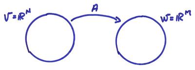
Matrix Transformations
Let A:RN
![]() RM with inner products
RM with inner products
![]() .
.
These will be called the usual inner products. Vectors will be represented by columns and A by an M x N matrix aij, i = 1,M, j = 1,N. (M is the number of rows (first index), N is the number of columns (second index)). A can be written

R(A) is the vector space spanned by the columns of A, and Nperp(A) is the vector space spanned by rows of A. The “rank” of a matrix A is the number of linearly independent columns of A (or the number of independent rows of A as well).
We want to show that the columns of A span R(A) and the rows of A span Nperp(A). Let
![]()
where ei
are the standard basis in RN
specified as

Then,

Let ai be the ith column of the matrix A

then,
![]()
with ![]() Thus, the range of A,
R(A), is spanned by the columns of A. Let
Thus, the range of A,
R(A), is spanned by the columns of A. Let

then,

If ![]() , then Av = 0,
and
, then Av = 0,
and ![]() . Then,
. Then, ![]() is perpendicular to
all bi, the rows of
the matrix A. Thus,
is perpendicular to
all bi, the rows of
the matrix A. Thus, ![]() is spanned by rows of A.
is spanned by rows of A.
Now the rank of A is noted as r and is equal to the dimension of the space spanned by the columns of A, as well as the dimension of the space spanned by the rows of A. Thus, the rank r is
r(A) = Dim {R(A)} = Dim {Nperp(A)}
Ex) Let

with A:R3 ![]() R3.
R3.
Find the basis for the range R(A).
1) Check Det A. If Det A = 0, then the columns of A are linearly dependent. Since Det A = 0, choose the basis for R(A) as

Thus, the rank of A is equal to 2.
Choose as a basis for Nperp(A) the independent rows of A as
(1 0 1)
(0 1 1)
To find N(A), use fact that V = N(A) + Nperp(A). Thus, for N(A), find all vectors perpendicular to Nperp(A).
Matrices are examples of linear transformations. Also, any linear transformation between finite dimensional vector spaces is “isomorphic” with a matrix.
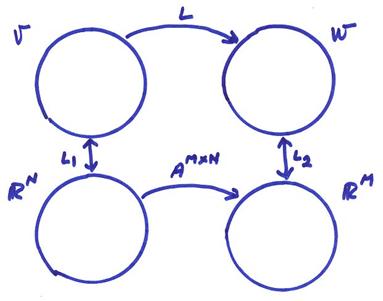
Use L1 to go from V to RN and L2 to go from W to RM. Then
L(v) = L2AL1(v)
where L1, L2 are just basis representations of vectors in V and W. Thus,
![]()
![]()
then,

and

Thus, A tells us how to map from basis functions in V to basis functions in W
