EAS 657
Geophysical Inverse Theory
Robert L. Nowack
Lecture 5
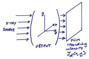
We first give an example for an X-ray imaging system
Transmitted photons either interact with matter or pass
through unaffected. Then, the number of
photons interacting with materials and removed from a beam, ![]() , in a region of thickness,
, in a region of thickness, ![]() , is
, is
![]()
where ![]() is linear attenuation
coefficient and N is total number of photons in the incident beam. This can be written as
is linear attenuation
coefficient and N is total number of photons in the incident beam. This can be written as
![]()
![]()
where L is the total thickness of the object. The intensity attenuation follows the same relationship as the number of photons. The intensity is the energy per unit area and can be expressed as the number of photons per unit area weighted by the energy per photon
![]()
For the most part, diffraction of the X-ray beams can be ignored resulting in straight ray paths of the beams. The classic X-ray picture can be thought of as a partial tomographic image where only one projection is used. The idea in tomography is to use many projections with different angles to reconstruct a 3-D estimation of the interior of a body.
In terms of log-intensity

This can be treated as a linear inverse problem in order to
reconstruct ![]() (x,y,z),
the material absorption.
(x,y,z),
the material absorption.
When finite
wavelengths are involved, diffraction effects will strongly distort energy
estimates and thus the simple formula above will not hold. For example, in seismic/acoustics in the Earth’s
crust, the compressional wave speed is about 6 km/sec. From the relation ![]() , for different waveperiods, the
wavelengths are
, for different waveperiods, the
wavelengths are
T = 1 sec (1 HZ) ![]() = 6.0 km
= 6.0 km
T = .1 sec (10 HZ) ![]() = .6 km
= .6 km
T = .01 sec (100 HZ) ![]() = 0.6 km
= 0.6 km
For small enough wavelengths compared to the heterogeneity scales, an approximate solution along ray trajectories can still be written as
![]()
where A is a complicated
combination of focusing and absorption and ![]() is the travel time
along the ray trajectory.
is the travel time
along the ray trajectory.
In the time domain,
![]()
with
![]()
where T(x) is a time of flight measurement and s = v-1 is the slowness inversely related to the speed along the ray trajectory.
If we assume really large heterogeneities and small variations of the slowness, s, then the ray paths will be approximately straight.
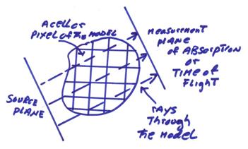
In order to reconstruct the structure of the object, the pixel or cell parameters of the model can be estimated from integrated parameters along rays (this is also called a Radon Transform). These types of linear integrals work best for large scale model parameters. For small scale model parameters, a different type of linearization has been shown to work best in estimating small scale scatterers. In physics, this is called Born Inversion and in exploration geophysics it is called seismic migration. This will be discussed more in a later lecture.
Ex) A 1-D time of flight problem in an elongated rock sample is shown below.
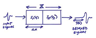
Assume we just have two pixels in our model (obviously we can break our model into finer and finer pixels giving more model unknowns).
![]()

The process of discretization reduces an infinite dimensional problem (here on the real line [0,X]) to a finite dimensional problem.
In our case, we can write a matrix problem As = T

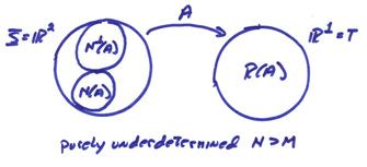
R(A) is spanned by the columns of A and [1] is a basis. Nperp(A) is spanned by the rows and a basis is (1,1). N(A) is spanned by (1,-1). This is an onto mapping since R(A) = T and Rperp(A) = {0}. But it is obviously not 1-1 since the dimensions of s and T are different.
This is a purely underdetermined problem and if we use the formula which determines the components of the solution vector in Nperp(A), we get the minimum norm solution. Then,
![]()
Note that N(A*) = Rperp(A) = Rperp(AA*) = {0}.
Since in this case Rperp(A) = {0}, the matrix AA* (this is a square MxM matrix and in this case is 1x1) is invertible and
sII = A*(AA*)-1T
where sII is the component of the solution in Nperp(A). Now,
![]()
and
![]()
Then,

The minimum norm solution is obviously in Nperp(A)
spanned by ![]() where
where
![]()
Since Nperp(A) is spanned by ![]() , the minimum norm solution will be an average large scale
solution along the ray. Since the null
space is spanned by
, the minimum norm solution will be an average large scale
solution along the ray. Since the null
space is spanned by ![]() , we can add a slowness component to s1 and subtract an equal amount to form s2 and still obtain the same
travel time T.
, we can add a slowness component to s1 and subtract an equal amount to form s2 and still obtain the same
travel time T.
Assume we
have a constraint on the problem that ![]() find
smallest norm solution. Let,
find
smallest norm solution. Let,
![]() where
where ![]()
then,

This can be shown to satisfy the original equation,
As = T.
We will also have in this problem non-negativity constraints on s1 and s2 which will also limit the nullspace components of the solution
If integrated time of flight or absorption data along many ray trajectories of different orientations are collected, then the properties of the object for individual pixels can be uniquely determined from the projections or integrations along rays. The inverse problem of finding the model parameters at the individual pixels from the projections involves two steps. The first step backprojects the data along the rays. This is similar to the case above for one ray, but for the general case it is done along many rays of different orientations. The second step is a filtering step resulting in a filtered backprojection image. In the Fourier domain, this can be formulated in terms of the Fourier slice theorem (see Herman, C.T. (1980), Image Reconstructions from Projections: The Fundamentals of Computerized Tomography, Academic Press). The mathematics of this procedure was first described by Radon in the early part of the 20th century. It was applied in radio astronomy by Bracewell in the 1950’s and by Cormack for X-ray tomography in the 1960’s. For his work in tomography, Cormack won the Nobel Prize in Medicine.