EAS 657
Geophysical Inverse Theory
Robert L. Nowack
Lecture 6
Spectral
Decompositions and Singular Value Decompositions
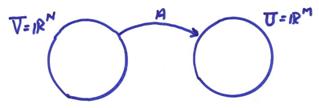
We will first investigate finite dimensional mappings represented by square matrices
A:RN ![]() RN
RN
An eigenvector for the operator A is a vector whose direction remains unchanged upon the operation of operator A. Thus
![]()
where ![]() is a scalar called the
eigenvalue associated with u. Also, a zero eigenvalue can be associated
with the equation
is a scalar called the
eigenvalue associated with u. Also, a zero eigenvalue can be associated
with the equation
Au = 0
The eigenvalue, ![]() , is in general a complex scalar. u
is an eigenvector if
, is in general a complex scalar. u
is an eigenvector if ![]() with
with ![]() . Thus, (A-
. Thus, (A-![]() I) must be singular (not invertible). This will occur when Det(A-
I) must be singular (not invertible). This will occur when Det(A-![]() I) = 0. Det(A-
I) = 0. Det(A-![]() I) = 0 is called the characteristic equation and can be
factored as
I) = 0 is called the characteristic equation and can be
factored as
![]()
Ex) A:R2 ![]() R2 A =
R2 A = ![]()

Back solving this for the eigenvectors for A gives
![]()
We now
define the eigenvectors of the adjoint operator A*, w, and the corresponding eigenvalues ![]() . Since transposing
doesn’t change the determinant, the eigenvalues of A* are the complex conjugates
of the eigenvalues of A. Thus
. Since transposing
doesn’t change the determinant, the eigenvalues of A* are the complex conjugates
of the eigenvalues of A. Thus
![]()
Now since
![]() ,
,
if ui is an eigenvector of A and wj is an eigenvector of A*, then
![]()
Thus, if ![]() , then wj
must be perpendicular to ui. This is called the biorthogonality relation for eigenvectors of A and A* for distinct
, then wj
must be perpendicular to ui. This is called the biorthogonality relation for eigenvectors of A and A* for distinct ![]() .
.
Theorem: Let ![]() be distinct eigenvalues
of A. Then the corresponding
eigenvectors of A are independent. Thus
(u1, u2, … uN) can be used as a
basis for U. This is a major utility of
eigenvectors.
be distinct eigenvalues
of A. Then the corresponding
eigenvectors of A are independent. Thus
(u1, u2, … uN) can be used as a
basis for U. This is a major utility of
eigenvectors.
For each eigenvector then,
![]()
or putting all the eigenvectors into one equation

If the ui are all linearly independent (which is not guaranteed for repeated eigenvalues), then
![]()
and
![]()
This is called a spectral representation of the linear operator A with independent eigenvectors. Of course, if the eigenvectors are not independent, then one cannot perform the inverse of M.
Ex) ![]()
but
![]()
Thus, for this example, u1 is not distinct from u2 and a spectral decomposition cannot be performed on this matrix.
Matrices of the form

are called Jordan
Blocks and have all eigenvectors for ![]() the same. For these type of matrices, spectral
decompositions using eigenvectors cannot be performed.
the same. For these type of matrices, spectral
decompositions using eigenvectors cannot be performed.
This type of problem, with eigenvectors used as a basis for square operators, can be extended for more general decomposition of operators using the singular value decomposition. However, eigenvector expansions are very useful for self adjoint operators where
A* = A.
In this case, ![]() . Thus, the
eigenvalues for any self adjoint (Hermitian
matrix) operator are real. Also, the eigenvectors of A and A* are the
same. Thus, ui = wi. In this case, for
. Thus, the
eigenvalues for any self adjoint (Hermitian
matrix) operator are real. Also, the eigenvectors of A and A* are the
same. Thus, ui = wi. In this case, for ![]() then, ui is perpendicular uj. Thus, the eigenvectors are directly orthogonal
and not biorthogonal.
then, ui is perpendicular uj. Thus, the eigenvectors are directly orthogonal
and not biorthogonal.
We have only showed this for distinct eigenvalues, but in fact, for an arbitrary case of repeated eigenvalues, we can always construct an orthonormal set of eigenvectors for a Hermitian matrix. (Hermitian matrices will never reduce to Jordan Blocks.) We can, therefore, always perform spectral decompositions for self adjoint operators (for Hermitian matrices)!
Any matrix with orthonormal columns is called unitary and has the property that
M-1 = M*
M*M = MM* = I
Thus, since M is unitary for a symmetric Hermitian matrices, then
![]()
Directly in terms of the eigenvectors for a square Hermitian Matrix A,
![]()
where ![]() denotes an outer
product. This is called the spectral theorem. Thus,
denotes an outer
product. This is called the spectral theorem. Thus,
![]()
This scales each ui
by ![]() and the projection of x on each ui.
and the projection of x on each ui.
For all nondefective square matrices (no Jordan Blocks), we can define functions of matrices as
![]()
where ![]() is the ith power of
the matrix A and
is the ith power of
the matrix A and ![]() is a function of the
matrix. This corresponds to the scalar
expansion for
is a function of the
matrix. This corresponds to the scalar
expansion for ![]() as
as
![]()
Since
![]()
then

In general, for a nondefective square matrix,

This is called Sylvester’s theorem.
Ex) Most linear physical systems can be written as a system of first order differential equations
![]()
The formed solution to this is eAt where A is a matrix. But what is eAt? By analogy to the 1-D case
![]() has a solution
has a solution ![]()
Using Sylvester’s theorem,

Solving systems of differential equations is another major use of eigenvectors and eigenvalues.
Ex) The stress “tensor” is a matrix quantity at a point in space where one index relates to the coordinate face on which the traction acts and the second index is the traction vector component.
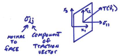
The traction vector acting on a plane with normal ![]() can be written
can be written
![]() sum on j
sum on j
Now we want
to find the vectors ![]() such that
such that
![]()
or
![]() eigenvector problem
eigenvector problem
On these faces, only normal tractions act. ![]() are the principle
stress directions and
are the principle
stress directions and ![]() are the principle
stresses. The
are the principle
stresses. The ![]() define three
orthonormal directions since
define three
orthonormal directions since ![]() is symmetric, then
is symmetric, then
![]()
where M is  are the principle
directions, and
are the principle
directions, and  is a diagonal matrix
of principle stresses.
is a diagonal matrix
of principle stresses.
Generalized Matrix
Analysis
Only Hermitian matrices are guaranteed not to have problems in standard eigenvector/eigenvalue analysis and non-square matrices are excluded. Fortunately, many differential operators are self adjoint which allow this sort of symmetric matrix analysis.
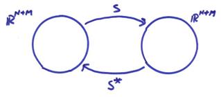
To avoid problems in other cases, Lanczos (1959) devised a trick of imbedding a general non-square matrix A within a larger Hermitian matrix
![]()
S is now Hermitian and, therefore, has a complete set of eigenvectors and real eigenvalues.
If A is an MxN matrix
Then S is an (M+N) x (M+N) matrix. Thus,
Solutions
to ![]() define the
eigenvectors and eigenvalues for S.
Since we are interested in A, we will split the eigenvectors w into parts
define the
eigenvectors and eigenvalues for S.
Since we are interested in A, we will split the eigenvectors w into parts

where ![]() is length M and
is length M and ![]() is length N. Then
is length N. Then
![]()
This can also be written
![]()
This is a coupled eigenvalue problem through A and its adjoint A*. Note that if
![]()
is an eigenvector for ![]() , then
, then
![]()
is an eigenvector for ![]() .
.
The eigenvalues of S are found from
![]()
If there are 2P non-zero eigenvalues, then

Since the eigenvector set for S is orthogonal (or made orthogonal for repeated eigenvalues)
![]()
then

and

Thus, ui is perpendicular to uj and vi is perpendicular to vj where
![]()
![]()
We will normalize these to 1.
The
eigenvalues, ![]() , separate the coupled eigenvalue problem into
, separate the coupled eigenvalue problem into
![]()
![]()
The ![]() , i = 1, N-P, span the nullspace N(A) of A, thus
, i = 1, N-P, span the nullspace N(A) of A, thus
![]()
and correspondingly ![]() , i = 1, M-P, span the nullspace N(A*), thus
, i = 1, M-P, span the nullspace N(A*), thus
![]()
Since these equations are now decoupled, we can now organize
the eigenvectors of S. for nonzero ![]()


where P is the rank of A and also the dimension of Nperp(A) or R(A). For the zero eigenvalues,


Thus, by playing this trick of constructing S, we have been able to span the domain and range of A by eigenvector-like orthonormal vectors.
Now lets look again at the coupled eigenvector problem
![]()
Operate on the first equation by A*, then
![]()
and the second equation by A, then
![]()
where A*A is an (NxN) matrix and AA* is an (MxM) matrix. These are ordinary eigenvalue problems for (A*A) and (AA*). Note that since
(x, A*Ay) = (A*Ax, y)
(x, AA*y) = (AA*x, y)
both A*A and AA* are self adjoint (Hermitian matrices). Thus {u},
i = 1,M, and {v}, i = 1,N, form
complete eigenvector systems for the operators {AA*} and {A*A}. The number of non-zero positive eigenvalues ![]() is P where
is P where ![]() .
.
Define

These are the “singular values” and are always positive real numbers. We can also separate the eigenvectors into matrices.


and
![]()
where ![]() are the non-zero
eigenvalues for A*A and AA*. Now let
are the non-zero
eigenvalues for A*A and AA*. Now let
V = [Vp, V0]
U = [Up, U0]
Since the columns of V and U form complete orthonormal sets of eigenvectors for A*A and AA*, then V* = V-1 and U* = U-1 are unitary matrices. Thus,
UU* = U*U = IMxM
VV* = V*V = INxN
For the reduced set Up (a MxP matrix) and Vp (a NxP matrix) by orthogonality of the colums of Up, then
Up* Up = Ipxp Vp* Vp = Ipxp
where Up* is PxM, Up is MxP, Vp*
is PxN and Vp is NxP. But in
general, UpUp* ![]() IMxM
(unless P = M, and VpVp*
IMxM
(unless P = M, and VpVp* ![]() INxN
(unless P = N).
INxN
(unless P = N).
Now we want to assemble this into one representation for A.


where A is MxN, Vp is NxP, Up is MxP,
V0 is Nx(N-P), A* is NxM, ![]() is PxP, and U0
is
is PxP, and U0
is
Mx(M-P). We can then write
![]()
and

If we multiple this through, then the only non-zero term is
![]()
This is called the singular value decomposition of the operator or matrix where


The columns of Up and Vp are orthonormal vectors that span R(A) and Nperp(A) respectively. This is a general representation of any matrix regardless of whether it is square or non-square, or whether it is complete or defective. The subspaces spanned by U0 and V0 can be thought of as “blindspots” not illuminated by A.
Ex) Let
v1 + v2 = 1
v3 = 2
-v3 = 1
This can be written in matrix form as

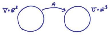
where A:R3 ![]() R3
R3
Now,


In U space: ![]() , i = 1, 2, 3. The
eigenvalues are found from
, i = 1, 2, 3. The
eigenvalues are found from

![]()
Thus,
![]()
The u1
and u2 eigenvectors
are found by solving AA*ui
= 2ui for u1 and u2 and normalizing ![]() Thus,
Thus,

The third eigenvalue is zero, so

Thus,

Now we can use a shortcut to solve for the Vp space
by ![]()

Find the V0 space vector by solving A*Av3 = 0

then,

This is the singular value decomposition of the matrix A.