EAS 657
Geophysical Inverse Theory
Robert L. Nowack
Lecture 7
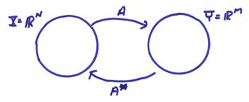
The Generalized Inverse Operator
The singular value decomposition of a general linear operator can be written
![]()
where

are the eigenvectors of (AA*) associated with the non-zero eigenvalues and span R(A) = R(AA*).

are eigenvectors of (A*A) associated with the non-zero eigenvalues that span Nperp(A) = N(A*A). The singular values are,

where ![]() are the non-zero
eigenvalues of A*A, AA*. Also,
are the non-zero
eigenvalues of A*A, AA*. Also, ![]() are the non-zero
positive eigenvalues of the larger matrix
are the non-zero
positive eigenvalues of the larger matrix ![]() .
.
Now, we are interested in solving the linear matrix equation
Ax = y
We have previously classified problems Ax = y into
the following categories.
1) N(A) = {0}, Rperp(A) = {0}. For this case, A is then one-to-one and invertible and
![]()
Recall that
![]()
with
![]()
where Det Mij is the minor formed by deleting row
i and column j of A. A is in invertible
if Det A ![]() 0.
0.
In terms of the SVD, M=N=P, and
![]()
where Up
is MxP, ![]() is PxP, and
is PxP, and ![]() is PxN. Because Up and Vp now
completely span the domain and range, then
is PxN. Because Up and Vp now
completely span the domain and range, then
Up*Up = UpUp* = 1 Vp*Vp = VpVp* = 1
thus,
![]()
The solution is then,
![]()
(Note in general, ![]() for
for ![]()
Note that for the case where N(A) = 0 and Rperp(A) = 0, instead of explicitly computing A-1, we can also factor A as
A = L U
where L is a lower triangular matrix  and U is an upper triangular
matrix
and U is an upper triangular
matrix  .
.
Then, Ax = y can be written as L Ux
= y.
Now solve ![]() and
and ![]() by back substitution. This is called Gaussian elimination. The number of algebraic operation counts is
by back substitution. This is called Gaussian elimination. The number of algebraic operation counts is
![]()
backsubstitution ~ N2
We can derive this factorization of A with householder transformations and QR algorithms later. Note, to directly compute, A-1 is on the order of N3 operations which is larger. Thus, inverses are computed only when they are needed.
2) Purely
underdetermined systems. For this case,
a nonunique solution to Ax = y results where
N(A) ![]() 0
0
We know from the previous sections that if Rperp(A) = {0}, then the minimum norm solution is
XMN = A*(AA*)-1y
Recall that (ABC)* = C*B*C*, then
![]()
If U0 = {0} or Rperp(A) = {0}, then
![]()
Thus,
![]()
This is the generalized inverse for purely underdetermined case in terms of the SVD.
3a) Purely overdetermined system. For this case, the system is incompatible, but the solution is unique, where
Rperp(A) ![]() 0, N(A) = {0}
0, N(A) = {0}
We need to find the best approximation solution. From previous sections, this can be found from the least squares solution
![]()
If V0 = {0} or N(A) = {0}, then
![]()
thus
![]()
3b) Both
N(A) ![]() 0 and Rperp(A)
0 and Rperp(A)
![]() 0. For this case, we want to find the best
approximation – minimum norm solution since the system is incompatible and the
solution is nonunique. In this case, the
generalized inverse can directly be written in terms of the SVD as
0. For this case, we want to find the best
approximation – minimum norm solution since the system is incompatible and the
solution is nonunique. In this case, the
generalized inverse can directly be written in terms of the SVD as
![]()
The solution to Ax = y for all cases can then be written as
![]()
where V0 are the basis vectors spanning the
nullspace N(A). The first term on the
right is the minimum norm solution and the second term results from the
nullspace required by additional constraints to the problem. However, in many cases, if it is known that
either Rperp(A) = {0} or N(A) = {0}, it may be computationally more
efficient to compute the specialized forms for ![]() .
.
But for the
specialized solutions, there may be numerical difficulties when dealing with
small eigenvalues for (A*A) and (AA*) since these have eigenvalues that are
squared ![]() . For the earlier
example, Ax = y, then
. For the earlier
example, Ax = y, then

then,

and

Thus,

and

This is the best approximation – minimum norm solution.
Resolution Matrix
The best approximation-minimum norm solution is given by
![]()
Let x by any solution to y = Ax, then
![]()
where ![]() is called the resolution matrix and is the operator
that determines the relationship between any possible solution x and the particular solution, xg. In terms of the SVD, R can be written
is called the resolution matrix and is the operator
that determines the relationship between any possible solution x and the particular solution, xg. In terms of the SVD, R can be written
![]()
Thus,
![]()
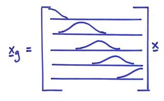
where Vp includes the vectors in Nperp(A)
and ![]() are coefficients. This operator projects x onto the Vp space resulting in the minimum norm
solution in Nperp(A). Note
that R is an NxN matrix. If P = N, then
are coefficients. This operator projects x onto the Vp space resulting in the minimum norm
solution in Nperp(A). Note
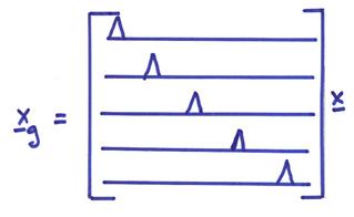
that R is an NxN matrix. If P = N, then ![]() is an identity matrix.
is an identity matrix.
If a particular row of R is “![]() -like” with a one on the main diagonal, then that component
of xg is called
“well resolved”. If a row of R is not “
-like” with a one on the main diagonal, then that component
of xg is called
“well resolved”. If a row of R is not “![]() -like”, then certain components of xg are not well resolved. Since
-like”, then certain components of xg are not well resolved. Since

then,
![]()
For P=N, then R is ![]() –like and xg
= x.
–like and xg
= x.
The so-called Backus-Gilbert Method finds solutions that minimize various norms of the “off diagonal” components of R in order to obtain a generalized inverse and solution xg.
As an example of computing R, consider

with

Thus,

Note that the “trace” of R (sum of diagonal elements) = P, which is the rank of A. This shows that the x3 component is well separated and uniquely resolved, but only the average of the components x1 and x2 is well resolved. The value of the Rii is often used to quantify the degree of resolution of model parameter xi.
For an
incompatible system Ax ![]() y, then
y, then
![]()
where yg is component of the data in R(A). Then, we have
![]()
or
![]()
where Up are vectors in R(A) and ![]() are the coefficients. N is called the relevancy matrix and is MxM. If N=I, then all the data are sensitive to
the operator A and P=M.
are the coefficients. N is called the relevancy matrix and is MxM. If N=I, then all the data are sensitive to
the operator A and P=M.
Next we look at the errors in the
solution. Assume the data have errors ![]() , then
, then
![]()
This is the part of the error in the solution mapped from
the data errors ![]() , but doesn’t include the nonuniqueness ambiguity. Let’s look at the “covariance matrix”. Recall that the average of a random variable x is
, but doesn’t include the nonuniqueness ambiguity. Let’s look at the “covariance matrix”. Recall that the average of a random variable x is

where f(x) is called the probability density function or pdf.
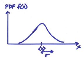
The variance ![]() measures the spread about
the mean <x>, where
measures the spread about
the mean <x>, where

The covariance of two random variables is defined as

where f(x,y) is the joint pdf of random variables x and y.
If x and y are formally independent and uncorrelated, then f(x,y) = f(x)f(y) and <xy> = <x><y>; then ![]() = 0.
= 0.
For a vector of random variables

then we can define a covariance matrix about the mean as

where ![]() is the outer product.
is the outer product.
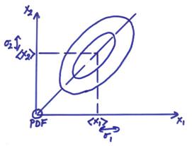
2-D Example
The linear correlation coefficient between two random variables x1 and x2 is

In the extreme cases, ![]() , then x1
and x2 are linearly
related to one another. The figure below
shows the pdf of two random variables with a positive correlation coefficient.
, then x1
and x2 are linearly
related to one another. The figure below
shows the pdf of two random variables with a positive correlation coefficient.
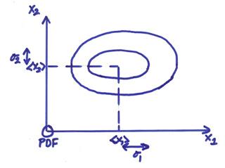
The figure below shows an example of the pdf of two random
variable x1 and x2 which are uncorrelated
with ![]() = 0.
= 0.
The covariance matrix of two random variables can be written

and is a symmetric matrix.
1) The
diagonal elements of C measure the “width”  of the joint pdf along
the axes.
of the joint pdf along
the axes.
2) The off-diagonal elements of C indicate the degree of correlation between pairs of random variables.
For the special case of Gaussian or normally distributed random variables, the mean and variances are all that are needed to specify the entire pdf.
1) 1-D case
![]()
2) N-D case
![]()
For our
case, ![]() and
and ![]() . The model covariance
matrix can be written as
. The model covariance
matrix can be written as

where ![]() is the average. Now
is the average. Now
![]()
![]()
where ![]() = Cd is the
data covariance. If all
= Cd is the
data covariance. If all ![]() are identically
distributed and uncorrelated independent random variables, then
are identically
distributed and uncorrelated independent random variables, then
![]()
where ![]() is the individual
component of the data variances Then,
is the individual
component of the data variances Then,
![]()
where ![]() is called the unit
covariance matrix for the solution due to errors in the data. It amplifies data errors back to the model.
is called the unit
covariance matrix for the solution due to errors in the data. It amplifies data errors back to the model.
Summary
For each of
the cases, we will write down ![]() , R, N, and Cu.
, R, N, and Cu.
1) Rperp(A) = {0}, N(A) = {0}. This is the invertible case where ![]()
Cu = A-1A-1* = (A*A)-1
R = A-1A = I
N = AA-1 = I
2) Rperp(A) = {0}, N(A) ![]() {0}. This is the purely undetermined case and we
want the minimum norm solution.
{0}. This is the purely undetermined case and we
want the minimum norm solution.
![]()
![]()
![]()
![]()
3a) Rperp(A) ![]() {0}, N(A) = {0}. This is the purely overdetermined case and we
want the best approximation or least squares solution.
{0}, N(A) = {0}. This is the purely overdetermined case and we
want the best approximation or least squares solution.
![]()
![]()
![]()
![]()
3b) Rperp(A) ![]() {0}, N(A)
{0}, N(A) ![]() {0}. This is the general case and we want the best
approximation – minimum norm solution.
{0}. This is the general case and we want the best
approximation – minimum norm solution.
![]() (This is the most
general form)
(This is the most
general form)
![]()
![]()
![]()
![]()
Note that

Tradeoffs Between
Variance and Resolution
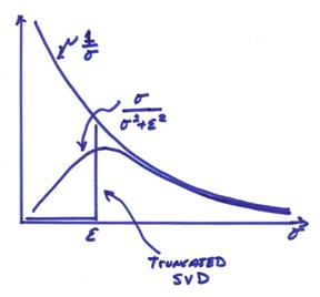
If ![]() is small but non-zero,
then
is small but non-zero,
then ![]() will be large. Thus, even if the data errors
will be large. Thus, even if the data errors ![]() are small, a small
are small, a small ![]() will magnify these tremendously
and will disturb the solution.
will magnify these tremendously
and will disturb the solution.
We would
like to eliminate the effects of small singular values on the solution. We could just eliminate small ![]() ’s, but this would reduce P resulting in a poorer resolution
matrix R (or a less
’s, but this would reduce P resulting in a poorer resolution
matrix R (or a less ![]() -like resolution).
Thus, if we want stability in the solution due to perturbations or
errors in the data, we must sacrifice resolution or resolving power of the
various components of the solution.
Recall
-like resolution).
Thus, if we want stability in the solution due to perturbations or
errors in the data, we must sacrifice resolution or resolving power of the
various components of the solution.
Recall
![]()
and for uncorrelated data errors ![]() , then
, then
![]()
For our example case,

then,

The cross correlation of x1 and x2 is
 resulting in perfect
correlation between x1 and
x2
resulting in perfect
correlation between x1 and
x2
Also,

Thus, ![]() . Note that Cx
is not a measure of the absolute error in the model since the true model
can also differ by any amount in N(A).
Recall the original observation equation x1 + x2
= 1 which does not require x1
= x2 which is only the
minimum norm solution.
. Note that Cx
is not a measure of the absolute error in the model since the true model
can also differ by any amount in N(A).
Recall the original observation equation x1 + x2
= 1 which does not require x1
= x2 which is only the
minimum norm solution.
Thus, Cx will underestimate the true model errors if
1) There exists a non-zero N(A).
2) There are additional modeling errors.
3) If nonlinearities exist and the problem was linearized.
There is also a tradeoff between ![]() –like resolution and the covariance of the solution resulting
from the data errors
–like resolution and the covariance of the solution resulting
from the data errors
As a note
on notation, we have used ![]() for the singular
values
for the singular
values
 these are the singular
values of matrix A
these are the singular
values of matrix A
where
![]() where
where ![]() are the eigenvalues of
A*A and AA* for i=1,P
are the eigenvalues of
A*A and AA* for i=1,P
We also use ![]() and
and ![]() for variances of
random variables x1 and x2, as well as
for variances of
random variables x1 and x2, as well as ![]() and
and ![]() for the variances of
the data and model parameters. You need
to watch carefully for the context that these symbols are used.
for the variances of
the data and model parameters. You need
to watch carefully for the context that these symbols are used.
The R (resolution) and N (relevance) are matrices which are just projection operators, thus,
![]()
![]()
The unit covariance operator is ![]() . The data covariance is
. The data covariance is
![]() .
.
For independent identically distributed data, then

The model errors resulting from data errors are then
![]()
For ![]() , then
, then ![]() as shown before.
as shown before.
The Approximate
Generalized Inverse and Damped Least Squares
The generalized inverse takes care of any singularities due to zero singular values. But, in practice, we can have severe difficulties with small, but non-zero singular values, especially with numerical round-off errors.
One way
around this is to set a cutoff in the singular values and place all singular
value vectors with ![]() into an extended null
space
into an extended null
space ![]() . A very similar
effect can be attained without resorting to SVD. by a procedure called
“damping”. This involves solving the
extended system
. A very similar
effect can be attained without resorting to SVD. by a procedure called
“damping”. This involves solving the
extended system

This is formally overdetermined where the first M rows are
just the system Ax = y. The last N rows are the system Ix ~ 0. These last equations try to force the
solution x to zero. The constant ![]() relatively weights the
equations Ax = y with equations that force x as close as possible to
zero. For
relatively weights the
equations Ax = y with equations that force x as close as possible to
zero. For ![]() , one gets the original system. For
, one gets the original system. For ![]() , then x goes
to zero.
, then x goes
to zero.
Solving this extended system by standard least squares results in
![]()
![]()
and
![]()
this is the damped least squares solution. Using the SVD, then

and

Note that

since [VpV0] is complete and orthonormal. Then,

and
![]()


This is the damped least squares operator written in terms of the SVD.
The figure below shows the effect of truncating the singular values in SVD or by filtering the singular values smoothly using damped least squares.
The
resolution operator ![]() for damped least
squares becomes
for damped least
squares becomes

For increasing ,![]() reduces the overall resolution which now only approximates
to
reduces the overall resolution which now only approximates
to ![]() , but is reasonably close for small
, but is reasonably close for small ![]() .
.
The approximate
unit covariance operator ![]() for damped least
squares becomes
for damped least
squares becomes

and with ![]() , then
, then
![]()
Thus, increasing ![]() artificially reduces the
variance of the model parameters resulting from variance in the data.
artificially reduces the
variance of the model parameters resulting from variance in the data.
Note that the damped least squares solution is a straightforward way of adding constraints. We can add prior information as “data” to our problem in a similar fashion.
Ex) We want to solve Ax = y and we want the solution x to be as “smooth” as possible.
Let’s look at a 1-D model vector. An augmented system of equations can be written as

For this case, we will attempt to simultaneously solve Ax = y and force the first derivative to be small as (xi+1 – xi) ~ 0. The
weighting parameter is ![]() .
.
If we want to minimize the second derivative of the model, then

where the a values in the first and last rows depend on the boundary conditions.
We can also solve the equations in terms of data residuals as
![]()
where x0 is an initial solution where y0 = Ax0. The generalized solution can be written
![]()
![]()
or
![]()
In terms of the SVD,
![]()
For small errors in the data, and small errors in the initial solution, then
![]()
Forming the model covariance results in
![]()
or
![]()
where the first term results from errors in the data and the second term results from the projection of errors in the initial model onto N(A). If there were errors in the A matrix itself, this would result in a third term related to modeling errors.
If we assume a general damped inverse of the form
![]()
then
![]()
and
![]()
This will be further discussed in a later chapter (see also Tarantola, 1987).