

The November 14, 2007 M7.7 Northern
|
|
Larry BraileProfessor,
http://web.ics.purdue.edu/~braile/ November, 2007 |

1. Objectives: Illustrate the use of filtering of seismograms to learn more about earthquakes and wave propagation in the Earth and better understand the characteristics of signals contained in seismograms. Sometimes, filtering a seismogram is similar to searching for clues, like being a detective, to try to determine what happened to produce the signals observed on the seismogram!
2. Introduction: There are several interesting features of
seismograms from the November 14, 2007 M7.7
This document is available for viewing with a browser (html file) and for downloading as an MS Word document or PDF file at the following locations:
http://web.ics.purdue.edu/~braile/edumod/as1lessons/filtering/filtering.htm
http://web.ics.purdue.edu/~braile/edumod/as1lessons/filtering/filtering.doc
http://web.ics.purdue.edu/~braile/edumod/as1lessons/filtering/filtering.pdf
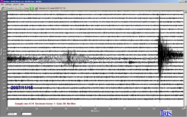
Figure 1. AmaSeis 24-hour screen
display for November 14-15, 2007 the WLIN AS-1 station showing the record of
the M7.7
Data and a summary map from
the USGS (http://earthquake.usgs.gov)
for this event and some aftershocks are given in Figures 2 and 3, and the WLIN
event data for the
3. Analysis of the WLIN
When I first saw the high
frequency arrival on the seismogram (Figures 6 and 7), I thought that it
probably was from an aftershock and that, because it occurred a short time
after the M7.7 earthquake, it hadn’t yet been identified and located. A day or two later, the suspected aftershock
still had not shown up on the USGS earthquake list, so I started looking at
some other seismograms (both AS-1 records available on SpiNet and some global
network records downloaded using the IRIS WILBER tool). There were several potential aftershock
signals on these seismograms in the approximate time range of the high
frequency arrival on the WLIN seismogram.
I tried picking the arrival times of the suspected aftershock arrivals
on several seismograms and locating the event using standard earthquake
location techniques. Nothing worked very
well, so I went back to the original WLIN record and considered other options
for the source of the high frequency arrival.
Because the arrival shows up on the WLIN record and other seismograms,
it is possible that the arrival is a later arriving phase from the
The arrival time of the high frequency phase on the WLIN seismogram closely matched the expected time for the PKPPKP phase – a raypath that travels from the earthquake focus through the Earth’s mantle and outer core and reflects off the surface on the far side of the Earth and then travels again through the mantle and outer core finally arriving at a station within about 90 degrees distance from the earthquake epicenter (an illustration will be provided later in this discussion). Because the match of travel time for this phase at only a single station is not very convincing evidence for identifying any unknown arrival, I examined other seismograms from large earthquakes in the range of zero to 90 degrees from the WLIN station to try to confirm that the high frequency arrival was actually the PKPPKP phase.
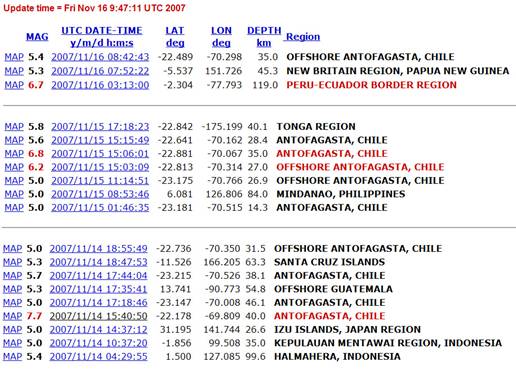
Figure 2. USGS earthquake list (http://earthquake.usgs.gov/eqcenter/recenteqsww/Quakes/quakes_big.php)
November 14-16, 2007.
4. The PKPPKP Phase on WLIN Seismograms: I found several WLIN seismograms from large earthquakes (a large event is needed as the PKPPKP phase has a very long travel path compared to the direct P arrival and thus has much smaller amplitude, as seen in Figure 7) in the appropriate distance range. I high-pass filtered the seismograms and measured the difference in travel times between the PKPPKP and the first P arrivals and compared these times with theoretical times calculated from a standard Earth velocity model. Three of the additional seismograms are shown in Figures 8, 9 and 10. Additional information on filtering AS-1 seismograms (or other sac-file records) with the AmaSeis software can be found in Section 3.5 of the Using AmaSeis tutorial: http://web.ics.purdue.edu/~braile/edumod/as1lessons/UsingAmaSeis/UsingAmaSeis.htm.
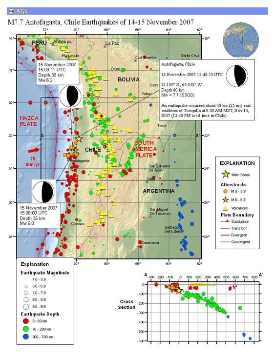
Figure 3. USGS summary map and information for the M7.7
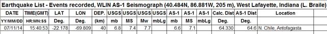
Figure 4. WLIN station information for November 14,
2007
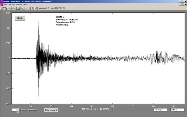
Figure 5. AmaSeis seismogram display
for November 14, 2007 the WLIN AS-1 station showing the seismogram of the M7.7
(http://web.ics.purdue.edu/~braile/edumod/as1lessons/filtering/0711141552WLIN.sac).
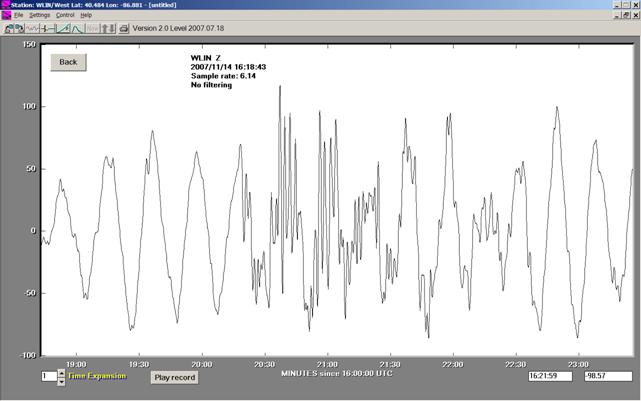
Figure 6. Close-up view of the surface wave arrival. Note the “unusual” high frequency energy.
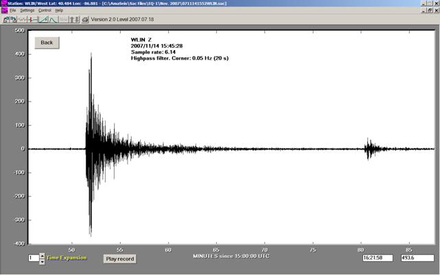
Figure 7. High pass filtered (0.5Hz) seismogram of the
M7.7
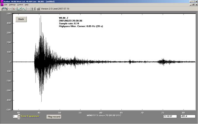
Figure 8. High pass filtered (0.5Hz) seismogram of the
M8.4 June 23, 2001
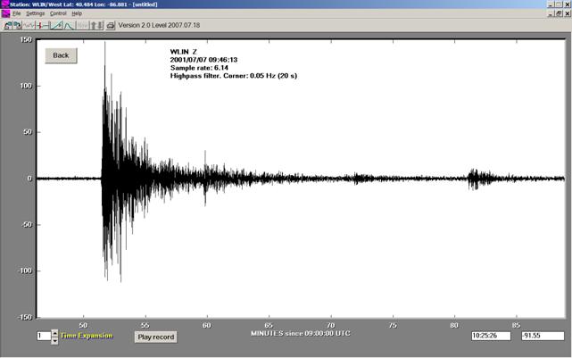
Figure 9. High pass filtered (0.5Hz) seismogram of the
M7.6 July 7, 2001
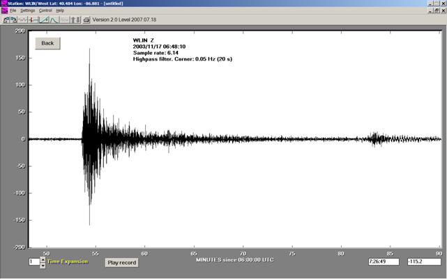
Figure 10. High pass filtered (0.5Hz) seismogram of the
M7.8 November 17, 2003
The event information for the selected WLIN PKPPKP seismograms is shown in the table in Figure 11. A comparison of the observed and calculated PKPPKP minus P travel times for nine WLIN seismograms is given in the table in Figure 12. Links to the seismograms (sac format) are given in the table in Figure 13. The close match between the observed and calculated times for seismograms from a significant range of distances confirms the identification of the PKPPKP phase as the source of the high frequency energy arriving about 25-31 minutes after the first P arrival in these seismograms. The travel time relationship for the P and PKPPKP phases is illustrated in the travel time curves in Figure 14. I also analyzed the seismograms from AS-1 stations AZAZ, SHCA and VVNY (obtained from SpiNet - http://www.scieds.com/spinet/) and found that the observed PKPPKP-P travel times matched the theoretical times to within a few seconds. Note that as the distance increases, the PKPPKP minus P travel time decreases (Figure 12). This travel time relationship is similar to a few other phases represented on the travel time curves in Figure 14, and results from the PKPPKP phase initially “going the opposite direction” or “taking the long way” to the station. We will also see this effect later when we further examine the surface wave arrival. The raypath for the PKPPKP phase is illustrated in Figure 15.
Note that to confirm the identification of the PKPPKP phase, we needed to analyze more than one seismogram. However, the phase was visible on individual seismograms through a simple filtering process available using the AmaSeis software.
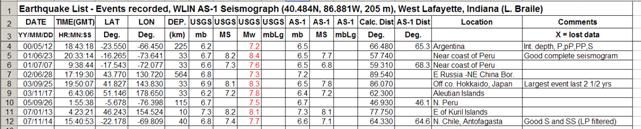
Figure 11. Table of earthquake
information for WLIN PKPPKP seismograms.
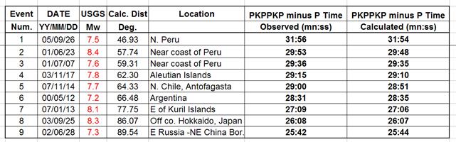
Figure 12. Table of travel times
for WLIN PKPPKP seismograms. The
information is sorted by increasing epicenter-to-station distance (given in
degrees geocentric angle). Observation
of PKPPKP at smaller distances is more difficult because of the small number of
large events within about 45 degrees of WLIN.
An explanation of distances measured in geocentric angle is available in
the Interpreting Seismograms tutorial at:
http://web.ics.purdue.edu/~braile/edumod/as1lessons/InterpSeis/InterpSeis.htm.
Figure 13. Table of links for
sac files for PKPPKP seismograms. The
event numbers correspond to the list in the Table in Figure 12. To use, download the seismograms into a
folder (name it “
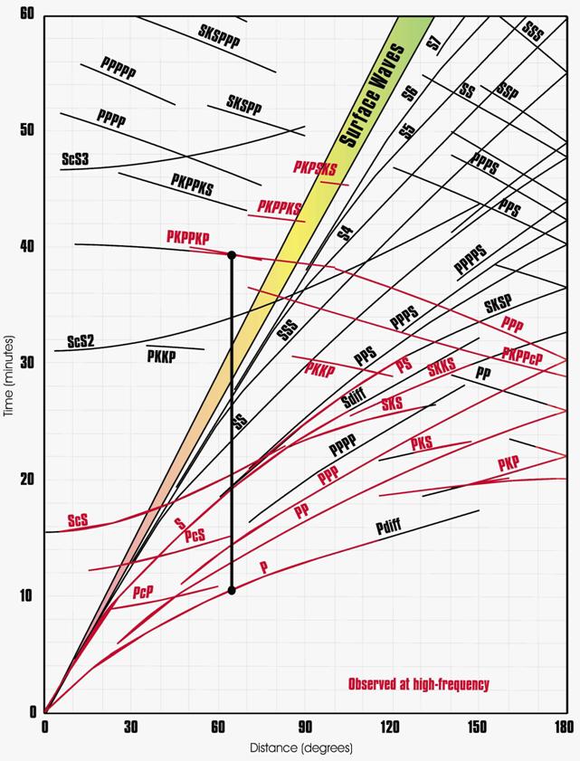
Figure 14. Standard travel-time
curves (http://neic.usgs.gov/neis/travel_times/
) for various phases (arrivals) for the Earth.
The dots show travel times for the
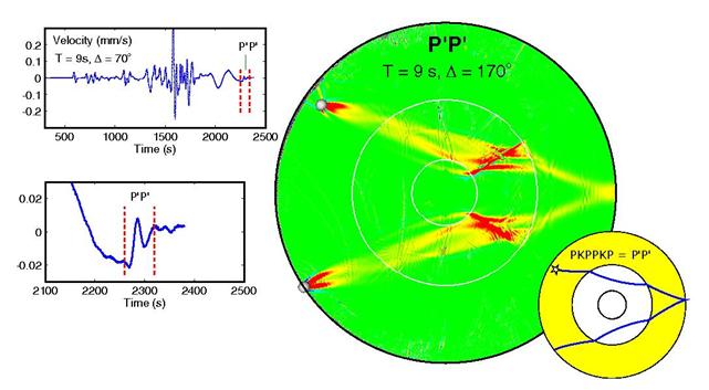
Figure 15. Illustration of the
PKPPKP phase (also called P’P’). The
seismograms show a weak long-period PKPPKP arrival calculated from a standard
Earth velocity model. The large Earth
cross section illustrates the complex raypaths
(from the calculated numerical model) of the wave energy that
contributes to the PKPPKP phase arrival.
The small Earth cross section shows the simplified PKPPKP raypath. Note that the P phase would travel more
directly from the earthquake (the star in the small Earth cross section) to the
recording station (in this example, about 60 degrees from the epicenter).
( from: http://www.agu.org/focus_group/SEDI/main/images/PKPPKP.html)
5. Calculating the Magnitude of
the Northern Chile Earthquake from the WLIN Seismogram: The epicenter-to-station distance for the
http://web.ics.purdue.edu/~braile/edumod/as1lessons/UsingAmaSeis/UsingAmaSeis.htm.
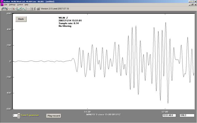
Figure 16. Close-up view of the P-arrival for the
6. Identification of the S Arrival and Estimating the Epicenter-to-Station Distance from the S Minus P Time: The S minus P travel time method can be used to estimate the epicenter-to-station distance from a seismogram for earthquakes within about 110 degrees from the station. An S minus P earthquake location exercise is available at:
http://web.ics.purdue.edu/~braile/edumod/as1lessons/EQlocation/EQlocation.htm. Identification of the S arrival on AS-1 vertical component seismograms is sometimes difficult or impossible. However, for regional or more distant events, low-pass filtering the seismogram with a cutoff frequency of 0.5 Hz (2 s period) or 0.2 Hz (5 s period) often allows the S arrival to be recognized. Another filter in AmaSeis that is often effective is the “long period filter” developed by Bob McClure. Applying the long period filter (settings are: Natural Frequency/Period = 2 s, Q = 0.707, LP = 20 s) to the N. Chile WLIN seismogram (Figure 5) results in the filtered seismogram shown in Figure 17. Note the prominent arrival (recognized by large amplitude and a shift in frequency of the wave energy (to lower frequencies) at a time of about 60 minutes past 15:00 on the time scale. The surface wave energy is also enhanced by this filter.
Using the arrival time
picking tool in AmaSeis, one can select the arrival times of the P and S waves
on the filtered seismogram and then use the travel time curve tool to estimate
the epicenter-to-station distance as shown in Figure 18. When the seismogram is displayed in the
travel time curve window, one can use the mouse cursor to move the seismogram
on the screen until the P and S arrival times correspond to the first blue
(direct P) and green (direct S) curves. The
epicenter-to-station distance determined by the S minus P time for the
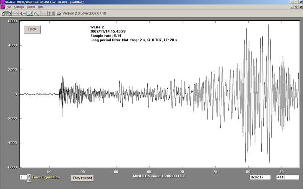
Figure 17. Long-period filtered
seismogram of the M7.7
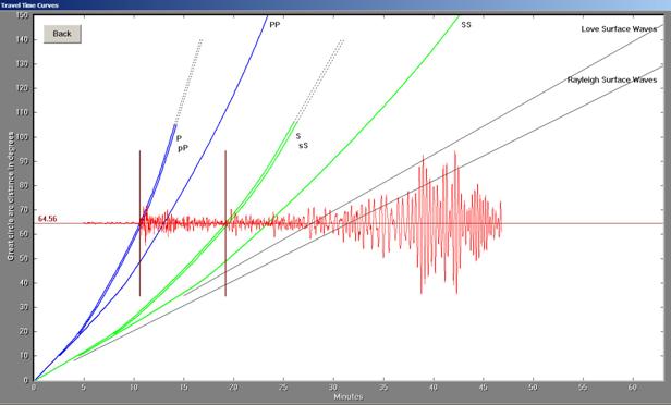
Figure 18. Long-period filtered seismogram displayed using the AmaSeis travel time curve tool.
7. Surface Waves Around the
World: In the process of examining
the WLIN N. Chile seismogram to see if there were aftershocks visible after
high-pass filtering (see section 3 above), I extracted a long (~ 3 hour)
seismogram for analysis (Figure 19). Two
aftershocks and a separate event (from
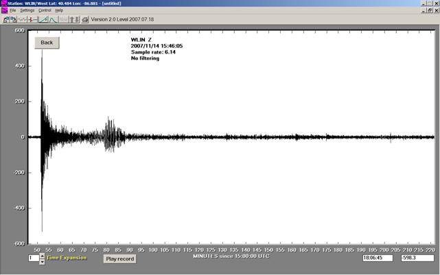
Figure 19. Three-hour seismogram
record for the
(http://web.ics.purdue.edu/~braile/edumod/as1lessons/filtering/0711141552WLINlong.sac).
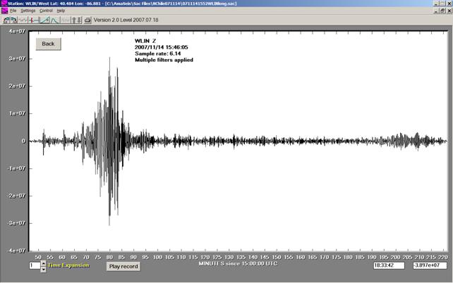
Figure 20. Long-period filtered
(three times), three-hour seismogram of the M7.7
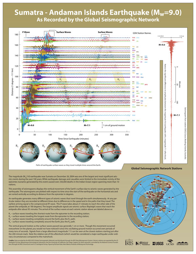
Figure 21. IRIS December 26,
2004
(http://www.iris.edu/about/publications.htm#p).
8. Examples of High- and Low-Pass Filtering: The long period surface waves and high frequency arrival (PKPPKP) visible on the WLIN N. Chile seismogram provide an excellent opportunity to illustrate the effects of filtering. Figure 22 shows the original and filtered seismograms for these phases. Note that the high-pass filter enhances the high frequency energy associated with the PKPPKP arrival and effectively removes most of the low-frequency surface wave energy. Similarly, the low-pass filter enhances the surface wave energy and effectively removes most of the high frequency energy.
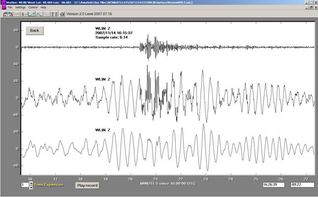
Figure 22. Example of seismogram
filtering. Middle trace is original WLIN
seismogram for the
Surface waves recorded at
teleseismic distances (greater than about 40 degrees), particularly surface
waves that have traversed oceanic regions, often display a very sinusoidal
(similar to a simple sine wave) character.
An example is the surface wave energy from the November 27, 2007 Solomon
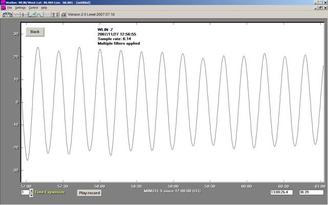
Figure 23. Surface waves from
the November 27, 2007 Solomon Islands earthquake recorded on the WLIN AS-1
seismograph. The seismogram has been
filtered twice with a low-pass filter (0.1 Hz cutoff frequency) to enhance the
surface wave energy
(http://web.ics.purdue.edu/~braile/edumod/as1lessons/filtering/0711271209WLIN.sac).
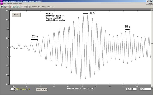
Figure 24. Surface waves from
the August 21, 2003 New Zealand earthquake recorded on the WLIN AS-1
seismograph. The seismogram has been
filtered twice with a low-pass filter (0.1 Hz cutoff frequency) to enhance the
surface wave energy
(http://web.ics.purdue.edu/~braile/edumod/as1lessons/filtering/0308211232WLIN.sac).
9. High-Pass Filtering to Identify Aftershocks: Moderate to large aftershocks are very common after major earthquakes. Sometimes, significant aftershocks occur within the first hour or so after a major event causing the P arrivals from the aftershocks to be recorded in the same time period as the surface waves for a distant event. An example is shown in Figure 25 for the November 15, 2006 M7.9 Kuril earthquake recorded at WLIN. After high-pass filtering the original seismogram, several prominent arrivals are visible on the filtered seismogram. Comparing arrival times of these events with the origin times of the aftershocks (the travel time from the epicentral area to WLIN is approximately 12 minutes) from the USGS list (Figure 26), we can identify at least six aftershocks. The aftershocks are numbered adjacent to the P arrival on the filtered seismogram and are listed in Figure 26. Arrivals labeled with a question mark on Figure 25 are uncertain as the possible corresponding events have small magnitude and would not be expected to be recorded at WLIN.
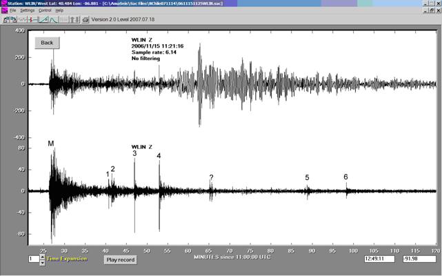
Figure 25. WLIN seismograms for
the November 15, 2006 M7.9 Kuril earthquake.
Upper trace is the original seismogram.
Lower trace is the high-pass filtered (cutoff frequency = 0.5 Hz)
seismogram (http://web.ics.purdue.edu/~braile/edumod/as1lessons/filtering/0611151125WLIN.sac).
The P arrival for the main shock is labeled “M”. The aftershocks are labeled with a number
corresponding to the events listed in Figure 26.
CATALOG D A T E ORIGIN ***COORDINATES** DEPTH pP STD *****M A G N I T U D E S****SOURCE YEAR MO DA TIME LAT LONG km DEV mb OBS Ms OBS CONTRIBUTED VALUESM PDE 2006 11 15 111413.57 A 46.592 153.266 10 G 1.07|6.5 99|7.8Z 99|8.30MwGCMT | |7.90MwGS | PDE 2006 11 15 112306.92*B 46.301 154.610 10 G 1.47|5.6 29| | | PDE 2006 11 15 112429.86 A 46.270 154.520 10 G 0.94|5.6 56| | | PDE 2006 11 15 112457.49*B 47.770 153.179 10 G 0.96|5.5 15| | | PDE 2006 11 15 112509 A 47.518 152.647 10 G 1.38|6.0 99| | |1 PDE 2006 11 15 112838.46 A 46.086 154.100 10 G 0.84|6.0 99| | |2 PDE 2006 11 15 112922.79 A 46.371 154.475 10 G 1.07|6.2 99| | | PDE 2006 11 15 113323.80 A 46.862 153.731 10 G 1.07|5.5 33| | |3 PDE 2006 11 15 113458.13 A 46.652 155.305 10 G 0.84|6.4 99| | |
PDE 2006 11 15 114003.87*B 47.673 151.525 10 G 1.10|5.3 15| | |4 PDE 2006 11 15 114055.05 A 46.483 154.726 10 G 0.90|6.4 99| |6.70MwGCMT | PDE 2006 11 15 114804.23*B 44.104 154.700 10 G 1.45|5.5 21| | | PDE 2006 11 15 115255.86*B 47.362 154.411 10 G 1.39|5.0 10| | | PDE 2006 11 15 120917.43 A 47.323 155.361 10 G 0.93|5.4 99| | | PDE 2006 11 15 121523.80 A 46.301 154.407 10 G 0.88|5.3 74| | |5 PDE 2006 11 15 121605.54 A 47.111 154.417 10 G 1.39|5.7 84| | |
5 PDE 2006 11 15 121644.15 A 46.195 154.668 10 G 0.82|5.9 99| | | PDE 2006 11 15 122304.07 A 46.789 153.395 10 G 1.12|5.0 39| | |6 PDE 2006 11 15 122615.76 A 47.421 153.861 10 G 0.79|5.7 99| | |
PDE 2006 11 15 122821.33 A 47.055 155.526 10 G 0.89|5.5 65| | |
Figure 26. Table of earthquake
information for the November 15, 2006 M7.9 Kuril earthquake and aftershocks (USGS
PDE catalog available from the earthquake search tool: http://neic.usgs.gov/neis/epic/epic.html). Identification of the main shock and
aftershock numbers have been added to the Table.
10. Filtering the AmaSeis Helicorder 24-Hour Display: To reduce some of the background noise and enhance the signals from distant earthquakes, John Lahr suggests (http://jclahr.com/science/psn/as1/filtering/index.html) trying the band-pass filter option on the AmaSeis display (helicorder). The original, unfiltered data are stored in the computer files, so one can turn the filter on or off and only the screen image is changed. An example is given in Figure 27. Notice that in the filtered signal, the high-frequency noise and microseisms are reduced and the long-period energy, especially the surface waves, are enhanced so that the earthquake signal is more visible.
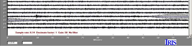
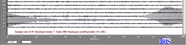
Figure 27. Partial helicorder
(24-hour screen) displays using AmaSeis for the November 27, 2007 M6.6
11. Suggestions for Additional Activities and Demonstrations of Filtering and Interpretation of Seismograms – See What You can Discover! Some suggestions for further exploration of seismograms and filtering are provided below. Some additional resources and information for the AmaSeis software, seismograph analysis and filtering are contained in the Using AmaSeis tutorial, the Interpreting Seismograms tutorial and in John Lahr’s web page on filtering:
http://web.ics.purdue.edu/~braile/edumod/as1lessons/UsingAmaSeis/UsingAmaSeis.htm
http://web.ics.purdue.edu/~braile/edumod/as1lessons/InterpSeis/InterpSeis.htm
http://jclahr.com/science/psn/as1/filtering/index.html. Information on the seismograms in sections 8, 9, 10 and 11 is contained in the Table in Figure 28.
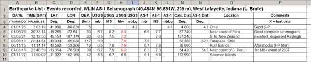
Figure 28. Table of earthquake
information for seismograms used in Sections 8,
9, 10 and 11.
a. Perform one or more of the filtering and analysis processes contained in sections 4 through 10 using the seismograms provided.
b. High pass filter (0.5 Hz cutoff frequency; or
2 s cutoff period) the June 13, 2005 M7.8
http://web.ics.purdue.edu/~braile/edumod/as1lessons/filtering/0506132254WLIN.sac.
c. Apply the long period filter to the Tarapaca,
d. Open the Tarapaca,
e. Use the November 11, 2006 M7.9
f. High pass filter (0.5 Hz cutoff frequency; or
2 s cutoff period) the June 23, 2001 M8.4
CATALOG D A T E
ORIGIN ***COORDINATES** DEPTH
pP STD *****M A G N I T U D E
S****
SOURCE
YEAR MO DA TIME
LAT LONG km
DEV mb OBS Ms
OBS CONTRIBUTED
VALUES
PDE
2001 06 23 203314.13
-16.264 -73.641 33
N 1.05|6.7 99|8.2Z
99|8.40MwHRV |
|8.30MwGS |
PDE
2001 06 23 205452.27?
-16.569 -73.728 33
N 1.38|5.4 11|
| |
PDE
2001 06 23 205607.21
-17.400 -72.166 33
N 0.99|5.8 39|
| |
PDE
2001 06 23 210539.17
-17.840 -71.348 33
N 1.04|5.8 36|
| |
PDE
2001 06 23 211614.87*
-17.322 -71.956 33
N 0.92|5.1 15|
| |
PDE
2001 06 23 211910.75
-17.047 -73.523 33
N 0.77|5.2 18|
| |
PDE
2001 06 23 212208.98*
-17.284 -72.237 33
N 1.38|5.4 11|
| |
PDE
2001 06 23 212735.71 -17.181
-72.641 33 N
0.92|6.1 84| | |
PDE
2001 06 23 213849.89
-17.115 -72.373 33
N 1.18|5.3 68|
| |
PDE
2001 06 23 214134.27*
-17.720 -71.054 33
N 0.99|5.0 4|
| |
PDE
2001 06 23 215453.81
-17.202 -72.632 33 N 1.05|5.1
44| | |
PDE
2001 06 23 215927.34
-16.756 -73.819 33
N 1.07|5.4 28|
| |
PDE
2001 06 23 222439.52
-16.645 -73.606 33
N 0.88|5.7 78|
| |
PDE
2001 06 23 223237.28
-17.602 -72.646 33
N 1.02|5.5 60|
| |
PDE
2001 06 23 231000.99
-16.767 -73.632 33
N 1.20|5.9 97|
| |
PDE
2001 06 23 234456.02 -16.751 -73.723
33 N 0.83|5.4
72| | |
PDE
2001 06 23 234913.88
-17.849 -71.579 33
N 0.87|5.6 83|
| |
Figure 29. Table of earthquake
information for the June 23, 2001 M8.4
g. Apply a high-pass filter (2 s cutoff period)
twice to the January 26, 2001 M4.2
h. High pass filter (0.5 Hz cutoff frequency; or
2 s cutoff period) the August 15, 2007 M8.0
http://web.ics.purdue.edu/~braile/edumod/as1lessons/filtering/0708152350WLIN.sac.
i. We have seen that seismic
signals from earthquakes have interesting frequency characteristics that can be
analyzed and interpreted using filtering, but we have not examined the
background noise that is always visible on the seismograph record. In this activity, we will use two noise
samples to analyze the background noise level, frequency content of the noise,
and the characteristics of microseisms. Background
noise is caused by environmental conditions such as high winds and ocean waves
and oscillations in coastal areas (microseisms), local human effects
(machinery, traffic, people walking), and distant small earthquakes and low
level shaking from recent large earthquakes long after the main seismic signals
have passed. Two screen displays of
background noise are shown in Figure
30. The first display is during a very
quiet time period while the second display is during a very noisy time period. A
sample of about 20 minutes long of the noise (Noise1) in the first example
(quiet background noise) has been extracted as a seismogram. Similarly, a sample of about 20 minutes long
of the noise (Noise2) in the second example (large background noise) has been
extracted as a seismogram. For each seismogram
noise sample, apply a 1 Hz low-pass filter to the data (to reduce the highest
frequency, relatively erratic oscillations in the noise seismograms. Note the noise level (amplitude, in digital
units) and appearance of the noise in the two samples. Extract about a 2 minute section of the
filtered noise samples and measure the period between two successive
peaks. Open the seismograms again and
filter them. Now use the Fourier
transform tool in AmaSeis to calculate the spectrum that displays the relative
amounts of amplitudes (or energy) in the signal at various frequencies. Compare the spectrum for each noise
sample. The noise in the second example
(Noise2) is primarily caused by microseisms that are commonly generated by wave
action and oscillations associated with storms along the east coast of
http://web.ics.purdue.edu/~braile/edumod/as1lessons/filtering/0707080220WLIN.Noise1.sac
http://web.ics.purdue.edu/~braile/edumod/as1lessons/filtering/0711032324WLIN.Noise2.sac.
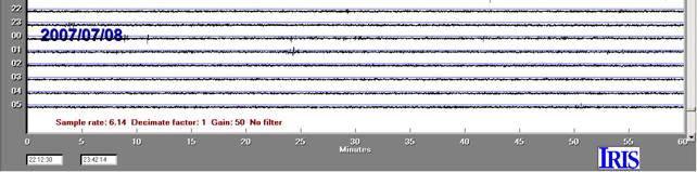
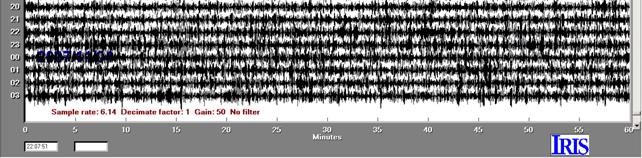
Figure 30. Partial helicorder
(24-hour screen) displays using AmaSeis for two time periods during the year
2007 recorded at the WLIN AS-1 seismograph station. Upper image
shows the one-hour traces of background noise from 22:00 on July 7 to
06:00 on July 8. Lower image shows the
one-hour traces of background noise from 20:00 on November 3 to 04:00 on
November 4. No filter has been applied
and the gain is 50 for both displays.
[1]  Last
modified December 26, 2007
Last
modified December 26, 2007
The web page for
this document is:
http://web.ics.purdue.edu/~braile/edumod/as1lessons/filtering/filtering.htm
Partial funding for this development provided by the National Science Foundation.
ã Copyright 2007. L. Braile. Permission granted for reproduction for non-commercial uses.