|
|
Seismic
Waves and the
Slinky: A Guide for Teachers Prof. Lawrence W.
BraileãDepartment of Earth, Atmospheric, and Planetary Sciences Purdue University West Lafayette, IN 47907-2051
|
|


Objectives: This teaching guide is designed to introduce the concepts of waves and seismic waves that propagate within the Earth, and to provide ideas and suggestions for how to teach about seismic waves. The guide provides information on the types and properties of seismic waves and instructions for using some simple materials – especially the slinky – to effectively demonstrate characteristics of seismic waves and wave propagation. Most of the activities described in the guide are useful both as demonstrations for the teacher and as exploratory activities for students. With several regular metal slinkys, and the modified slinky demonstrations described in this teaching guide, one can involve an entire class in observation of the demonstrations and experimenting with the slinkys in small groups. For activities that involve several people, such as the 5-slinky and human wave demonstrations, it is convenient to repeat the demonstrations with different groups of students so that each person will have the opportunity to observe the demonstration and to participate in it.
This tutorial is available for viewing with a browser (html file) and for downloading as an MS Word document or PDF file at the following locations:
http://web.ics.purdue.edu/~braile/edumod/slinky/slinky.htm
http://web.ics.purdue.edu/~braile/edumod/slinky/slimky.doc
http://web.ics.purdue.edu/~braile/edumod/slinky/slinky.pdf
A related PowerPoint presentation for seismic waves and the slinky is available for download at: http://web.ics.purdue.edu/~braile/new/SeismicWaves.ppt
 Last modified January
10, 2017
Last modified January
10, 2017
The web page for
this document is:
http://web.ics.purdue.edu/~braile/edumod/slinky/slinky.htm
Partial funding for this development provided by the National Science Foundation.
ã Copyright 2006-17. L. Braile. Permission granted for reproduction for non-commercial uses.
Contents
(click on topic to go directly to that section; use the red up arrows to return
to the list of contents):
4. Elasticity of a Spring Experiment
6. Slinky Demonstrations of P and S Waves
7. Illustration of
Energy Carried by the Waves
8.
Wave Propagation in All Directions
9.
Human Wave Demonstration – P and S Waves in Solids and Liquids
10.
Velocity of Wave Propagation Experiment
14.
Oscillations of the Whole Earth
15.
Seismic Waves in the Earth
Waves: Waves consist of a disturbance in materials (media) that carries energy and propagates. However, the material that the wave propagates in generally does not move with the wave. The movement of the material is generally confined to small motions, called particle motion, of the material as the wave passes. After the wave has passed, the material usually looks just like it did before the wave, and, is in the same location as before the wave. (Near the source of a strong disturbance, such as a large explosion or earthquake, the wave-generated deformation can be large enough to cause permanent deformation which will be visible after the disturbance has passed as cracks, fault offsets, and displacements of the ground.) A source of energy creates the initial disturbance (or continuously generates a disturbance) and the resulting waves propagate (travel) out from the disturbance. Because there is finite energy in a confined or short-duration disturbance, the waves generated by such a source will spread out during propagation and become smaller (attenuate) with distance away from the source or with time after the initial source, and thus, will eventually die out.
Waves are often represented mathematically and in graphs as sine waves (or combinations or sums of sine waves) as shown in Figure 1. The vertical axis on this plot represents the temporary motion (such as displacement amplitude A) of the propagating wave at a given time or location as the wave passes. The characteristics or properties of the wave – amplitude, wavelength, peaks, etc. – are illustrated in Figure 1.
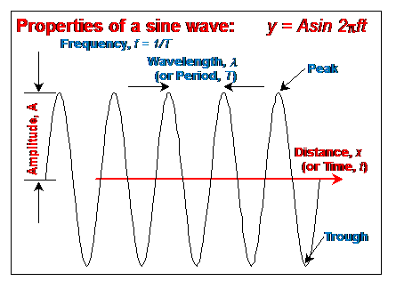
Figure 1. Properties of
a sine wave. The horizontal axis displays time or distance and the
vertical axis displays amplitude as a function of time or distance.
Amplitude can represent any type or measure of motion for any direction. Seismic
wave motion is commonly displayed with a similar plot, and sometimes the wave
itself looks very similar to the sine wave shown here.
Additional information on the properties of waves can be found in Bolt (1993, p. 29-30) or Rutherford and Bachmeyer (1995). Sometimes the actual wave looks very much like the representation in the graph (Figure 1). Examples are water waves and a type of seismic surface waves called Rayleigh waves. Commonly, propagating waves are of relatively short duration and look similar to truncated sine waves whose amplitudes vary with time.
Waves generated by a short duration disturbance in a small area, such as from an earthquake or a quarry blast, spread outward from the source as a single or a series of wavefronts. The wavefronts at successive times, and corresponding raypaths that show the direction of propagation of the waves, are illustrated in Figure 2. A good model for illustrating wave motion of this type is water waves from a pebble dropped in a still pond or pool. The disturbance caused by the pebble hitting the surface of the water generates waves that propagate outward in expanding, circular wavefronts. Because there is more energy from dropping a larger pebble, the resulting waves will be larger (and probably of different wavelength).
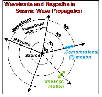
Figure 2. Wavefronts and raypaths for a seismic wave propagating from a source. Three positions (successive times) of the expanding wavefront are shown. Particle motions for P (compressional) and S (shear) waves are also shown. Raypaths are perpendicular to the wavefronts and indicate the direction of propagation of the wave. P waves travel faster than S waves so there will be separate wavefront representations for the P and S waves. If the physical properties of the material through which the waves are propagating are constant, the wavefronts will be circular (or spherical in three-dimensions). If the physical properties vary in the model, the wavefronts will be more complex shapes.
![]()
Return to list of contents
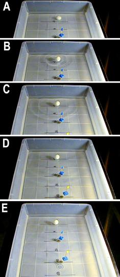
Waves in Water Experiment: Experiments with water waves in a small wave tank, consisting of a rectangular plastic storage box (about 60 to 120 cm long by 40 cm wide by 15 cm high; the exact size isn’t important); a plastic storage box designed to fit under a bed, available at discount department stores such as K-Mart, Wal-Mart and Target, with about 5 cm of water in it, can easily illustrate the common properties of water waves (Figure 3). Drops of water from an eyedropper or small spherical objects (a table tennis ball, a golf ball, or a small rubber ball works well) dropped onto the surface of the water are convenient sources. With the wave tank one can demonstrate that: the size (amplitude) of the waves is related to the energy of the source (controlled by the mass and drop height); the waves expand outward (propagate) in circular wavefronts; the wave height decreases and eventually dies out with distance away from the source (or with time after the source) because of spreading out of the wave energy over a larger and larger area (or volume); the waves have a speed (velocity) of propagation that can be measured by placing marks every 10 cm on the bottom of the tank and timing the wave with a stopwatch; the waves reflect off the sides of the tank and continue propagating in a different direction after reflection. About 3-4, small floating flags can be used to more effectively see the motion of the water as the wave passes. The flags are particularly useful for noting the relative amplitude of the waves as the degree of shaking of the flags is a visible indication of the size of the wave. Flags can be made from small pieces (~2x2x1 cm) of closed cell foam, styrofoam or cork. Place a small piece of tape on a toothpick and stick the toothpick into the foam or cork to create a floating flag (Figure 4) that is sensitive to waves in the water. By placing the flags in the wavetank at various distances from the source, one can easily observe the time of arrival and the relative amplitudes of the waves. A glass cake pan (Figure 5) can be used as small wave tank on an overhead projector. Waves generated by dropping drops of water from an eyedropper into about 2 cm of water in the tank will be visible on the screen projected from the overhead projector. The velocity of propagation, attenuation of wave energy, and reflection of waves are important concepts for understanding seismic wave propagation, so experimenting with these wave properties in the water tank is a very useful exercise. Additional suggestions for experiments with water waves are contained in Zubrowski (1994).
|
Figure 3. Large wave tank using a plastic storage container (75 liter "under bed" container). Distances in cm can be marked on the bottom of the container for convenient measurement of wave velocity from the distance and travel time. Small floating flags (Figure 4) are useful for identifying the time and relative amplitude of propagating water waves. The flags are made from small floats (about 2x2x1 cm rectangular blocks of closed cell foam, Styrofoam or cork) with a toothpick and piece of tape attached. The floating flags are very sensitive to wave motion in the wave tank. In this sequence of photos, taken every one-half second, one can see the waves propagating outward from the source. Lines drawn on the bottom of the tank are spaced at 10 cm. A. Source (a table tennis ball dropped from about 40 cm height) is just ready to hit the water surface. B. (~ 0.5 s after the source) Water waves have propagated from the source to about 10 cm distance. A circular expanding wavefront is visible and the wave height is larger than in the later photos. C. (~ 1.0 s) The wavefront has propagated to about 20 cm distance and the waves have decreased in amplitude. D. (~ 1.5 s) The wavefront has propagated to about 30 cm distance. E. (~ 2 s) The wavefront has propagated to about 40 cm distance and the wave amplitudes have decreased so much that they are difficult to see in this photo. The small floating flags are sensitive detectors (similar to seismometers) of the waves. Because the waves have traveled about 40 cm in 2 seconds, the velocity of propagation is about 20 cm/s or 0.2 m/s. |
|
|
|
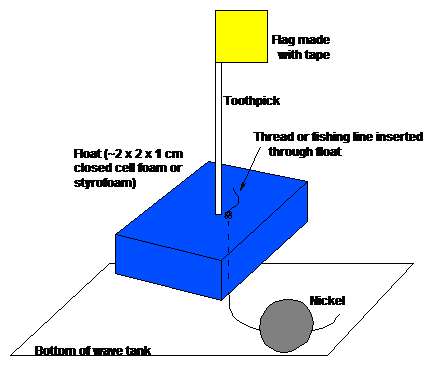
Figure 4. Small floating flags used to help detect the motion of water waves in a wave tank. The flags can be "anchored" using a length of thread and a nickel for a weight. The flags are sensitive to the motion caused by relatively small waves. By noting the degree of shaking of the flags, one can identify (approximately) large, medium and small (barely detectible) wave action. Be sure the water surface is calm (and the flags still) before initiating a water wave experiment.
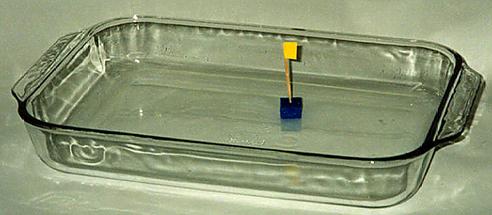
Figure 5. Small wave tank using a clear glass cake or baking dish. The dish with about 2 cm of water in it can be placed on an overhead projector so that wave propagation in the water can be seen on a screen.
![]()
Elasticity: Earth materials are mostly solid rock and are elastic, and thus propagate elastic or seismic waves in which elastic disturbances (deformation or bending or temporary compression of rocks) travel through the Earth. Elastic materials have the properties that the amount of deformation is proportional to the applied force (such as the stretching of a spring as masses are suspended from the spring), and that the material returns to its original shape after the force is removed (such as the spring returning to its original length after the masses are removed).
![]()
Elasticity of a Spring Experiment: An experiment designed to illustrate the elastic characteristics of a spring is shown in Figure 6. Measurements of the stretching of the spring as masses are added and removed are given in Table 1 and graphed in Figure 7. In contrast, some materials like most metals, are ductile. For example, if one bends a copper wire, it stays bent rather than returning to its original shape. One can even make a spring out of copper wire by wrapping the wire tightly around a cylindrical shaped object, such as a cardboard tube. Repeating the elasticity experiment with the copper wire spring will result in an elastic behavior (straight line relationships between the stretching and the amount of mass added) for small mass, and permanent deformation (stretching) for larger masses (the spring will not return to its original length as masses are removed). Data for the copper wire spring experiment can be tabulated, as in Table 1, and graphed, as in Figure 7. Because this experiment produces a very different stretching versus added mass curve, as compared to the regular spring example, it is useful to ask the students before the experiment what they expect the results to look like and then compare the actual results with their predictions.
|
|
|
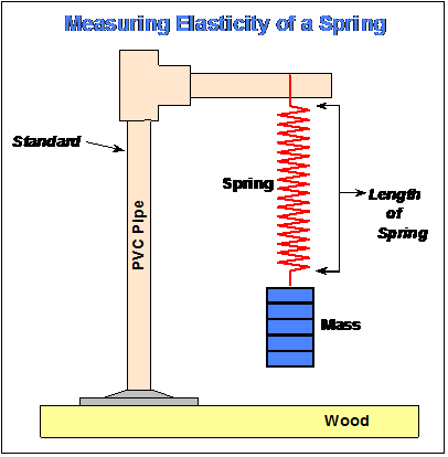
Figure 6. Schematic
diagram illustrating mass and spring apparatus for measuring the elasticity
(stretching of the spring as mass is added) of a spring.
Table 1. Observations of extension of a spring upon adding and removing masses.
|
Added Mass (g) |
Spring Extension (cm)* (adding masses) |
Spring Extension (cm)* (removing masses) |
|
0 |
0.0 |
0.3 |
|
100 |
3.7 |
3.6 |
|
200 |
7.7 |
7.5 |
|
300 |
11.4 |
11.4 |
|
400 |
15.3 |
15.1 |
*Spring
extension (stretching) is the length of the spring with mass attached minus the
length of the spring with no mass. Different springs have different
spring constants (elasticity) and will display different amounts of stretching
for a given amount of added mass. Many springs are tightly-wound and
require a small amount of force (suspended mass) to begin extending. For
these springs, one should use the difference between this initial suspended
mass and the total mass as the "added mass."
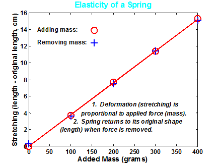
Figure 7. Graph showing measurements of elasticity of a spring. Measurements were made as mass was added and removed. The stretching of the spring is defined as the spring length (with added mass) minus the original length. Note that the extension versus mass data define a straight line. The slope of this line is related to the spring constant or elasticity of the spring. The two properties that characterize simple elasticity are described in the figure.
![]()
Seismic Waves: Unlike waves in water which are confined to a region very near to the water's surface, seismic waves also propagate through the Earth's interior. Because of the elastic properties of Earth materials (rocks) and the presence of the Earth's surface, four main types of seismic waves propagate within the Earth. Compressional (P) and Shear (S) waves propagate through the Earth’s interior and are known as body waves (Figure 8). Love and Rayleigh waves propagate primarily at and near the Earth's surface and are called surface waves. Wave propagation and particle motion characteristics for the P, S, Rayleigh and Love waves are illustrated in Figures 9-12. Further information and characteristics of these four kinds of seismic waves are given in Table 2.
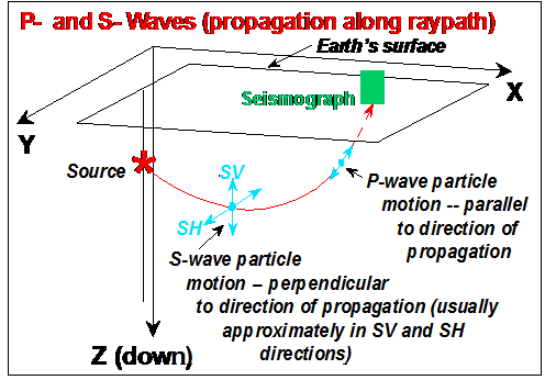
Figure 8. Raypath from the source to a
particular location on the surface for P- and S- wave propagation in a material
with variable velocity. P and S particle motion are shown. Because
major boundaries between different rock types within the Earth are normally
approximately parallel to the Earth's surface, S-wave particle motion is commonly
in the SV (perpendicular to the raypath and vertical) and SH perpendicular to
the raypath and horizontal) directions.
|
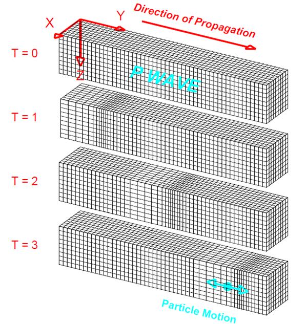
Figure 9. Perspective view of elastic P-wave propagation through a grid representing a volume of material. The directions X and Y are parallel to the Earth's surface and the Z direction is depth. T = 0 through T = 3 indicate successive times. The disturbance that is propagated is a compression (grid lines are closer together) followed by a dilatation or extension (grid lines are farther apart). The particle motion is in the direction of propagation. The material returns to its original shape after the wave has passed. |
|
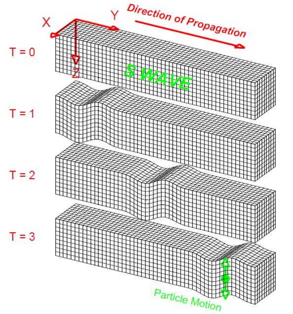
Figure 10. Perspective view of S-wave propagation through a grid representing a volume of elastic material. The disturbance that is propagated is an up motion followed by a down motion (the shear motion could also be directed horizontally or any direction that is perpendicular to the direction of propagation). The particle motion is perpendicular to the direction of propagation. The material returns to its original shape after the wave has passed. |
|
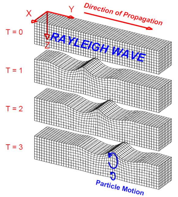
Figure 11. Perspective view of Rayleigh-wave propagation through a grid representing a volume of elastic material. Rayleigh waves are surface waves. The disturbance that is propagated is, in general, an elliptical motion which consists of both vertical (shear; perpendicular to the direction of propagation but in the plane of the raypath) and horizontal (compression; in the direction of propagation) particle motion. The amplitudes of the Rayleigh wave motion decrease with distance away from the surface. The material returns to its original shape after the wave has passed. |
|
Figure 12. Perspective view of Love-wave propagation through a grid representing a volume of elastic material. Love waves are surface waves. The disturbance that is propagated is horizontal and perpendicular to the direction of propagation. The amplitudes of the Love wave motion decrease with distance away from the surface. The material returns to its original shape after the wave has passed. |
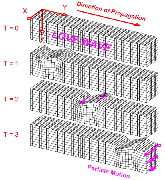
Table 2: Seismic Waves
|
|||
|
Type (and names) |
Particle Motion |
Typical Velocity |
Other Characteristics |
|
P,
Compressional, Primary, Longitudinal |
Alternating
compressions (“pushes”) and dilations (“pulls”) which are directed in the
same direction as the wave is propagating (along the raypath); and therefore,
perpendicular to the wavefront |
VP
~ 5 – 7 km/s in typical Earth’s crust;
>~ 8 km/s in Earth’s mantle and core; 1.5 km/s in water; 0.3 km/s in
air |
P
motion travels fastest in materials, so the P-wave is the first-arriving
energy on a seismogram. Generally smaller and higher frequency than the
S and Surface-waves. P waves in a liquid or gas are pressure waves,
including sound waves. |
|
S,
Shear, Secondary, Transverse |
Alternating
transverse motions (perpendicular to the direction of propagation, and the
raypath); commonly polarized such that particle motion is in vertical or
horizontal planes |
VS
~ 3 – 4 km/s in typical Earth’s crust;
>~ 4.5 km/s in Earth’s mantle; ~ 2.5-3.0 km/s in (solid) inner
core |
S-waves
do not travel through fluids, so do not exist in Earth’s outer core (inferred
to be primarily liquid iron) or in air or water or molten rock (magma).
S waves travel slower than P waves in a solid and, therefore, arrive after
the P wave. |
|
L,
Love, Surface waves, Long waves |
Transverse
horizontal motion, perpendicular to the direction of propagation and
generally parallel to the Earth’s surface |
VL
~ 2.0 - 4.5 km/s in the Earth depending on frequency of the
propagating wave |
Love
waves exist because of the Earth’s surface. They are largest at the
surface and decrease in amplitude with depth. Love waves are
dispersive, that is, the wave velocity is dependent on frequency, with low
frequencies normally propagating at higher velocity. Depth of
penetration of the Love waves is also dependent on frequency, with lower
frequencies penetrating to greater depth. |
|
R,
Rayleigh, Surface waves, Long waves, Ground roll |
Motion
is both in the direction of propagation and perpendicular (in a vertical
plane), and “phased” so that the motion is generally elliptical –
either prograde or retrograde |
VR
~ 2.0 - 4.5 km/s in the Earth depending on frequency of the
propagating wave |
Rayleigh
waves are also dispersive and the amplitudes generally decrease with depth in
the Earth. Appearance and particle motion are similar to water waves. |
Additional illustrations of P, S, Rayleigh and Love waves are contained in Bolt (1993, p. 27 and 37) and in Shearer (1999, p. 32 and 152). Effective animations of P and S waves are contained in the Nova video "Earthquake" (1990; about 13 minutes into the program) and of P, S, Rayleigh and Love waves in the Discovery Channel video "Living with Violent Earth: We Live on Somewhat Shaky Ground" (1989, about 3 minutes into the program) and in the animations and activities available at: http://web.ics.purdue.edu/~braile/edumod/waves/WaveDemo.htm.
![]()
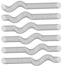
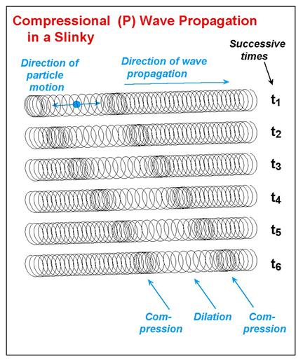
Slinky Demonstrations of P and S Waves: The P and S waves have distinctive particle motions (Figures 8, 9, and 10, and Table 2) and travel at different speeds. P and S waves can be demonstrated effectively with a slinky. For the P or compressional wave, have two people hold the ends of the slinky about 3-4 meters apart. One person should cup his or her hand over the end (the last 3-4 coils) of the slinky and, when the slinky is nearly at rest, hit that hand with the fist of the other hand. The compressional disturbance that is transmitted to the slinky will propagate along the slinky to the other person. Note that the motion of each coil is either compressional or extensional with the movement parallel to the direction of propagation. Because the other person is holding the slinky firmly, the P wave will reflect at that end and travel back along the slinky. The propagation and reflection will continue until the wave energy dies out. The propagation of the P wave by the slinky is illustrated in Figure 13.
|
Figure 13. Compressional (P) wave propagation in a slinky. A disturbance at one end results in a compression of the coils followed by dilation (extension), and then another compression. With time (successive times are shown by the diagrams of the slinky at times t1 through t6), the disturbance propagates along the slinky. After the energy passes, the coils of the slinky return to their original, undisturbed position. The direction of particle motion is in the direction of propagation. |
|
Figure 14. Shear (S) wave propagation in a slinky. A disturbance at one end results in an up motion of the coils followed by a down motion of the coils. With time (successive times are shown by the diagrams of the slinky at times t1 through t6), the disturbance propagates along the slinky. After the energy passes, the coils of the slinky return to their original, undisturbed position. The direction of particle motion is perpendicular (for example, up and down or side to side) to the direction of propagation. |
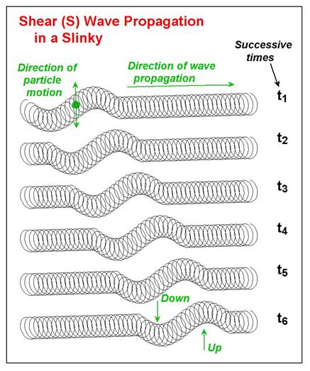
Demonstrating the S or Shear wave is performed in a similar fashion except that
the person who creates the shear disturbance does so by moving his or her hand
quickly up and then down. This motion generates a motion of the coils
that is perpendicular to the direction of propagation, which is along the
slinky. Note that the particle motion is not only perpendicular to the
direction of motion but also in the vertical plane. One can also produce
Shear waves with the slinky in which the motion is in the horizontal plane by
the person creating the source moving his or her hand quickly left and then
right. The propagation of the S wave by the slinky is illustrated in Figure
14. Notice that, although the motion of the disturbance was purely
perpendicular to the direction of propagation (no motion in the disturbing
source was directed along the slinky), the disturbance still propagates away
from the source, along the slinky. The reason for this phenomenon (a good
challenge question for students) is because the material is elastic and the
individual coils are connected (like the individual particles of a solid) and
thus transmit their motion to the adjacent coils. As this process
continues, the shear disturbance travels along the entire slinky (elastic
medium).
P and S waves can also be generated in the slinky by an additional method that reinforces the concept of elasticity and the elastic rebound theory which explains the generation of earthquakes by plate tectonic movements (Bolt, 1993, p. 74-77). In this method, for the P wave, one person should slowly gather a few of the end coils of the slinky into his or her hand. This process stores elastic energy in the coils of the slinky that are compressed (as compared to the other coils in the stretched slinky) similar to the storage of elastic energy in rocks adjacent to a fault that are deformed by plate motions prior to slip along a fault plane in the elastic rebound process. When a few coils have been compressed, release them suddenly (holding on to the end coil of the slinky) and a compressional wave disturbance will propagate along the slinky. This method helps illustrate the concept of the elastic properties of the slinky and the storage of energy in the elastic rebound process. However, the compressional wave that it generates is not as simple or visible as the wave produced by using a blow of one’s fist, so it is suggested that this method be demonstrated after the previously-described method using the fist.
Similarly, using this "elastic rebound" method for the S waves, one person holding the end of the stretched slinky should use their other hand to grab one of the coils about 10-12 coils away from the end of the slinky. Slowly pull on this coil in a direction perpendicular to the direction defined by the stretched slinky. This process applies a shearing displacement to this end of the slinky and stores elastic energy (strain) in the slinky similar to the storage of strain energy in rocks adjacent to a fault or plate boundary by plate tectonic movements. After the coil has been displaced about 10 cm or so, release it suddenly (similar to the sudden slip along a fault plane in the elastic rebound process) and an S wave disturbance will propagate along the slinky away from the source.
![]()
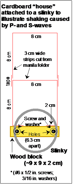
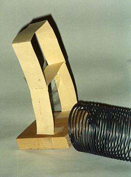
Illustration of Energy Carried by the Waves: The fact that the seismic waves (P or S) that propagate along the slinky transmit energy can be illustrated effectively by using a slinky in which one end (the end opposite the source) has a small wood block attached. The wood block has a cardboard model building attached to it as shown in Figures 15 and 16. As P or S wave energy that propagates along the slinky is transmitted to the wood block, the building vibrates. This model is a good demonstration of what happens when a seismic wave in the Earth reaches the surface and causes vibrations that are transmitted to houses and other buildings. By generating P, S-vertical and S-horizontal waves that transmit vibration to the model building, one can even observe differences in the reaction of the building to the different directions of motion of the propagating wave.
|
Figure 15. Diagram showing how to attach a slinky to the edge
of a small wood block with screws and washers. A cardboard
"building" is attached with tape to the wood block. The model
building is made from manila folder (or similar) material and is taped
together. The diagram is a side view of the slinky, wood block and
model building. When seismic waves are propagated along the slinky, the
vibrations of the cardboard building show that the wave energy is carried by
the slinky and is transmitted to the model building. |
|
Figure 16. Photograph
of slinky attached to a small wood block (Figure 15) and cardboard
"house." The slinky could also be attached to the bottom ot
the wood block to illustrate P- and S-waves propagating upwards and shaking
the building.
|
Wave Propagation in All Directions: An additional demonstration with P and S waves can be performed with the 5-slinky model. By attaching 5 slinkys to a wood block as shown in Figure 17, 5 people can hold the ends of the 5 slinkys (stretched out in different directions to about 3-4 m each). One person holds the wood block and can generate P or S waves (or even a combination of both) by hitting the wood block with a closed fist or causing the block to move quickly up and then down or left and then right. The purpose of this demonstration is to show that the waves propagate in all directions in the Earth from the source (not just in the direction of a single slinky). Attaching an additional slinky (with small pieces of plastic electrical tape) to one of the five slinkys attached to the wood block makes one slinky into a double length slinky which can be stretched out to 6-8 m. For one of the other four slinkys, have the person holding it collapse about half of the coils and hold them in his or her hands, forming a half slinky, stretched out about 1½ - 2 m. Now when a source is created at the wood block, one can see that the waves take different amounts of time to travel the different distances to the ends of the various slinkys. An effective way to demonstrate the different arrival times is to have the person holding each slinky call out the word "now" when the wave arrives at their location. The difference in arrival times for the different distances will be obvious from the sequence of the call of "now." This variation in travel time is similar to what is observed for an earthquake whose waves travel to various seismograph stations that are different distances from the source (epicenter). Although these two demonstrations with the five slinky model represent fairly simple concepts, we have found the demonstrations to be very effective with all age groups. In fact, the five slinky demonstrations are often identified as the "favorite" activities of participants.
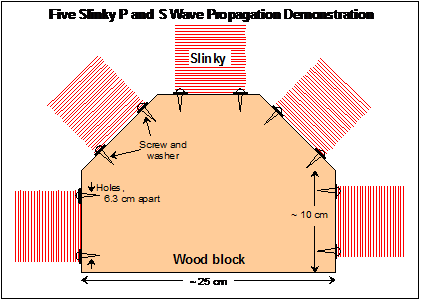
Figure 17. Diagram
showing how five slinkys can be attached to the edge of a wood block.
Photographs of the five slinky model are shown in Figures 18 and 19. When
the slinkys are stretched out to different positions (five people hold the end
of one slinky each) and a P or S wave is generated at the wood block, the waves
propagate out in all directions. The five slinky model can also be used
to show that the travel times to different locations (such as seismograph
stations) will be different. To demonstrate this effect, wrap a small
piece of tape around a coil near the middle of the slinky for one of the
slinkys. Have the person holding that slinky compress all of the coils
from the outer end to the coil with the tape so that only one half of the
slinky is extended. Also, attach an additional slinky, using plastic
electrical tape, to the end of one of the slinkys. Have the person
holding this double slinky stand farther away from the wood block so that the
double slinky is fully extended. When a P or S wave is generated at the
wood block, the waves that travel along the slinky will arrive at the end of
the half slinky first, then at approximately the same time at the three regular
slinkys, and finally, last at the double length slinky. The difference in
travel time will be very noticeable.
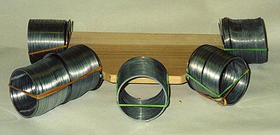
Figure 18. Photograph of
five slinky model.
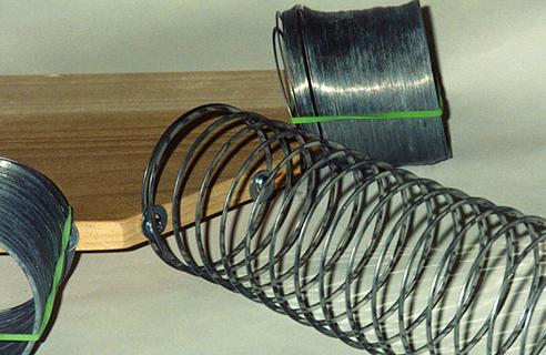
Figure 19. Close-up view of five slinky model showing attachment of slinky using screws and washers.
![]()
Human Wave Demonstration – P and S Waves in Solids and Liquids: This demonstration involves a class or group in simulating seismic wave propagation in solids and liquids. If you have 20 or more people in the group, half can perform the demo while the other half watches; then switch places. The concepts that are involved in this demonstration are very dramatically illustrated to the participants. Once they have done the human wave activity, they should always remember the properties of P and S waves propagating in both solids and liquids. Have about 10 people stand at the front of the room, side by side, with their feet about shoulder width apart. Instruct the group to not be too rigid or too limp when pushed from the side. They should give with the force that they will feel from the person next to them, but not fall over, and then return to their upright position. In other words, they should be "elastic". Have a “spotter” at the end of the line in case the last person begins to fall. (It is important to stress these instructions to the participants so that the demonstration will work effectively and so that participants do not fall over as the wave propagates down the line of people.)
To represent wave propagation in a solid, have each person put their arms over the shoulders of the person next to them (“chorus line style”; the “molecules” or "particles" of the solid are tightly bonded). Push on the person at the end of the line and the deformation (leaning to the side and then straightening up) will propagate down the line of people approximating a P wave (Figure 20). Note that the propagation down the line took some time (there is a velocity for the wave propagation) and that although each person was briefly subjected to a deformation or disturbance, the individuals did not move from their original locations. Also, the motion of each person as the wave passed was in the direction of propagation and that, as the wave passed, the people moved closer together temporarily (compression), and then apart (dilation) to return to their original positions.
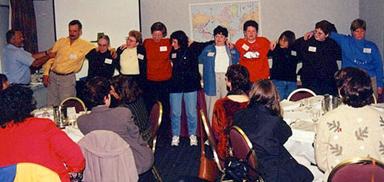
Figure 20. Human wave demonstration for the P wave in a solid. Instructor begins the P wave motion (in this case from left to right) in the line by pushing (compressing) on the first person in the line and then pulling the person back to an upright position.
For the S wave in a solid, make the first person at the end of the line bend forward at the waist and then stand up straight. The transverse or shear motion will propagate down the line of people (Figure 21). Again, the wave takes some time to propagate and each person ends up in the same location where they started even though a wave has passed. Also, note that the shear motion of each particle is perpendicular to the direction of propagation. One of the observers can time the P and S wave propagation in the human wave using a stopwatch. Because the shear wave motion is more complicated in the human wave, the S wave will have a slower velocity (greater travel time from source to the end of the line of people), similar to seismic waves in a solid.
|
Figure 21. Human wave demonstration for the S wave in a solid. The teacher starts the S wave motion (in this case propagating from right to left) in the line by causing the first person in the line to bend forward at the waist and then stand up straight. |

Next, to represent wave propagation in a liquid, have the people stand shoulder-to-shoulder, without their arms around each other. Push on the shoulder of the end person and a P wave will propagate down the line. The P wave will have the same characteristics in the liquid as described previously for the solid. Now, make the person at the end of the line bend forward at the waist – a transverse or shear disturbance. However, because the “molecules” of the liquid are more loosely bound, the shearing motion will not propagate through the liquid (along the line of people). The disturbance does not propagate to the next person because the liquid does not support the shearing motion. (Compare pressing your hand down on the surface of a solid such as a table top and on the surface of water and moving your hand parallel to the surface. There will be considerable resistance to moving your hand on the solid. One could even push the entire table horizontally by this shearing motion. However, there will be virtually no resistance to moving your hand along the surface of the water.) Only the first person in the line – the one that is bent over at the waist – should move because the people are not connected. If the next person bends, “sympathetically”, not because of the wave propagating, ask that person if he or she felt, rather than just saw, the wave disturbance, then repeat the demonstration for S waves in a liquid.
![]()
Velocity of Wave Propagation Experiment: Developing an understanding of seismic wave propagation and of the velocity of propagation of seismic waves in the Earth is aided by making measurements of wave speed and comparing velocities in different materials. For waves that travel an approximately straight line (along a straight raypath), the velocity of propagation is simply the distance traveled (given in meters or kilometers, for example) divided by the time of travel (or "travel time") in seconds. Using a stopwatch for measuring time and a meter stick or metric tape for measuring distance, determine the wave velocity of water waves in the wave tank, the P wave in the slinky, and the P wave in the human wave experiment. Also, determine the velocity of sound in air using the following method. On a playfield, measure out a distance of about 100 meters. Have one person with a stopwatch stand at one end of the 100 meter line. Have another person with a metal garbage can and a stick stand 100 meters away from the person with the stopwatch. Have the person with the stick hit the garbage can so that the instant of contact of the stick with the garbage can is visible from a distance. The person with the stopwatch should start the stopwatch when the stick strikes the can and stop it when the sound generated by the stick hitting the can is heard. The measured speed of sound will be the distance divided by the travel time measured on the stopwatch. (This measurement assumes that the speed of light is infinite – a reasonable approximation as the actual speed of light is about 3 x 10⁸ or 300 million meters/second, much faster than the speed of sound, and that the reaction time for the person operating the stopwatch is about the same for starting the watch when the can is struck and for stopping the watch when the sound is heard. The measurement should be repeated a few times to obtain an estimate of how accurately the measurement can be made. An average of the time measurements can be used to calculate the sound speed. The difference between the arrival of a light wave and associated sound is commonly used to determine how far away a lightning strike is in a thunderstorm. For example, because the speed of sound in air is about 330 m/s, if the difference in time between seeing a lightning strike and hearing the associated thunder is 3 seconds, the lightning is 1 km away; similarly, 6 s for 2 km away, etc.)
Make a list of the wave velocities (in m/s) for the water waves, slinky, human wave, and sound wave in air. (Measured wave speeds should be approximately 0.25-0.5 m/s for water waves in a wave tank, 2 m/s for the compressional human wave, 3 m/s for P waves in the slinky, and 330 m/s for sound waves in air.) Compare these wave velocities with the compressional wave velocity in the Earth which varies from about 1000 m/s for unconsolidated materials near the Earth's surface to about 14,000 m/s in the Earth's lowermost mantle (1 to 14 km/s). The seismic velocity in solid rocks in the Earth is controlled by rock composition (chemistry), and pressure and temperature conditions, and is found to be approximately proportional to rock density (density = mass/unit volume; higher density rocks generally have larger elastic constants resulting in higher seismic velocity). Further information on seismic velocities and a diagram showing seismic velocity with depth in the Earth is available in Bolt (1993, p. 143) and Shearer (1999, p. 3).
![]()
Attenuation
of Waves: To demonstrate the property of anelasticity, a model with
two slinkys can be constructed. Anelasticity is the absorption of energy
during propagation which causes waves to attenuate in addition to the
attenuation caused by the energy spreading out (for example, like the spreading
of water waves created by dropping a pebble into a pond). This effect is
an important concept in evaluating earthquake hazards and comparing the hazards
in two locations such as the western
Figure 22. Schematic
diagram illustrating the construction of a model using two slinkys (one with a
foam strip inside the coils of the slinky) that can be used to demonstrate the
concept of absorption of energy by material during propagation
(anelasticity). A photo of the slinky model for demonstrating absorption
is shown in Figure 23.
|
Figure 23. Slinky model used to demonstrate attenuation of waves by absorption of energy. |
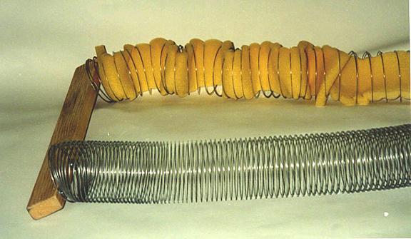
Small wood blocks and model buildings (Figure 15) can be attached to the free ends of both the regular slinky and the foam-lined slinky so that the wave energy that reaches the end of the slinky will be more visible for comparison. Extend each slinky about 3 m and cause P or S waves to be generated simultaneously in both slinkys by hitting the wood block (for P waves) or quickly moving the wood block vertically or horizontally (for S waves). The regular slinky will propagate the waves very efficiently while the slinky with the foam will strongly attenuate the wave energy (by absorbing some of the energy) as it propagates.
![]()
Reflection of Waves: The reflection of wave energy at a boundary between two types of materials can be demonstrated with slinkys by attaching a regular metal slinky to a plastic slinky (Figure 24). The attachment can be made with small pieces of plastic electrical tape. Generating P or S waves in the metal slinky will result in reflection of some of the wave energy at the boundary between the two stretched slinkys. Additional information about reflection and conversion of energy (S to P and P to S waves) of seismic waves at boundaries is given in Figure 25 and in Bolt (1993, p. 31-33)
|
Figure 24. Two slinkys – a metal slinky and a plastic slinky – attached together using small pieces of electrical tape. The two slinkys can be used to illustrate reflection and transmission of wave energy at a boundary between elastic materials with differing elastic properties. |
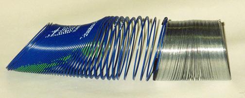
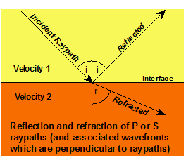
Figure 25. Reflection and refraction (transmission) of seismic waves (P or S waves) at an interface separating two different materials. Some energy is reflected and some is transmitted. The effect can be illustrated with two slinkys – one metal and one plastic – taped together. Waves traveling along one slinky are partially reflected at the boundary between the two types of slinkys. For seismic waves in the Earth, an incident P or S wave also results in converted S and P energy in both the upper material (reflected) and the lower material (transmitted). If the angle of approach of the wave (measured by the angle of incidence, i, or the associated raypath) is not zero, the resulting transmitted P and S raypaths will be bent or refracted at the boundary. A similar change in angle is also evident for the reflected, converted waves.
![]()
Surface Waves: The Love wave (Figure 12; Table 2) is easy to demonstrate with a slinky or a double length slinky. Stretch the slinky out on the floor or on a tabletop and have one person at each end hold on to the end of the slinky. Generate the Love wave motion by quickly moving one end of the slinky to the left and then to the right. The horizontal shearing motion will propagate along the slinky. Below the surface, the Love wave motion is the same except that the amplitudes decrease with depth (Table 2). Using the slinky for the Rayleigh wave (Figure 11, Table 2) is much more difficult. With a regular slinky suspended between two people, one person can generate the motion of the Rayleigh wave by rapidly moving his or her hand in a circular or elliptical motion. The motion should be up, back (toward the person generating the motion), down, and then forward (away from the person), coming back to the original location and forming an ellipse or circle with the motion of the hand. This complex pattern will propagate along the slinky but will look very similar to an S wave (compare Figures 10 and 11). Excellent illustrations of the wave motion of Love and Rayleigh waves can also be found in Bolt (1993, p. 37). Rayleigh wave motion also decreases with depth below the surface. Further details on the characteristics and propagation of Love and Rayleigh waves can be found in Bolt (1993, p. 37-41).
![]()
Oscillations of the Whole Earth: When a very large earthquake occurs, long period surface wave energy penetrates deep within the Earth and propagates all around the globe. At particular points around the globe, the timing between this wave energy (which just keeps circling the globe for many hours or even days before dying out or attenuating) results in constructive and destructive interference of the wave energy. The resulting oscillations at certain frequencies are called normal modes or free oscillations of the Earth and are vibrations of the whole Earth. Further information about Earth normal modes, the phenomenon of standing waves, and diagrams illustrating the modes of vibration of the whole Earth are available in Bolt (1993, p. 34-37 and 144-145) and Shearer (1999, p. 158-162).
![]()
Seismic Waves in the Earth: Seismic body waves (P and S waves) travel through the interior of the Earth. Because confining pressure increases with depth in the Earth, the velocity of seismic waves generally increases with depth causing raypaths of body waves to be curved (Figure 26). Because the interior structure of the Earth is complex and because there are four types of seismic waves (including dispersive surface waves), seismograms, which record ground motion from seismic waves propagating outward from an earthquake (or other) source, are often complicated and have long (several minutes or more) duration (Figures 27 and 28). An effective computer simulation that illustrates wave propagation in the Earth is the program Seismic Waves (Figure 29) by Alan Jones (see reference list). Using this program, which shows waves propagating through the interior of the Earth in speeded-up-real-time, one can view the spreading out of wavefronts, P, S, and surface waves traveling at different velocities, wave reflection and P-to-S and S-to-P wave conversion. The program also displays actual seismograms that contain arrivals for these wave types and phases. Exploring wave propagation through the Earth with the Seismic Waves program is an excellent follow-up activity to the seismic wave activities presented in this teaching guide.
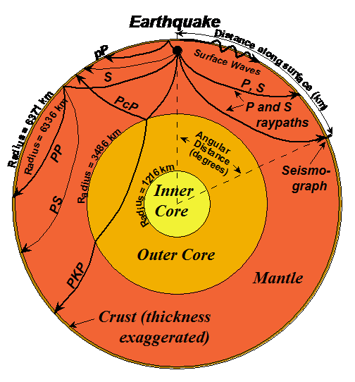
Figure 26. Cross
section through the Earth showing important layers and representative raypaths
of seismic body waves. Direct P and S raypaths (phases), including a
reflection (PP and pP), converted phase (PS), and a phase that travels through
both the mantle and the core (PKP). P raypaths are shown by heavy
lines. S raypaths are indicated by light lines. Additional
information about raypaths for seismic waves in the whole Earth and
illustrations of representative raypaths are available in Bolt (1993, p. 128-142)
and Shearer (1999, p. 49-60). Surface wave propagation (Rayleigh waves
and Love waves) is schematically represented by the heavy wiggly line.
Surface waves propagate away from the epicenter, primarily near the surface and
the amplitudes of surface wave particle motion decrease with depth.
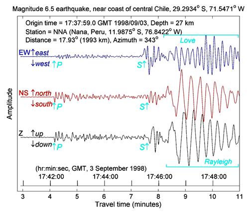
Figure 27. Seismograms
recorded by a 3-component seismograph at
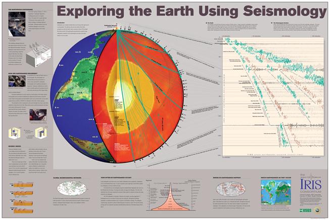
Figure 28. Model of the Earth's interior and selected raypaths for seismic wave propagation from the 1994 Northridge earthquake to seismograph stations around the world. Because of the existence of several types of seismic waves and the complex structure of the Earth's interior, many arrivals (phases) of seismic energy are present and are identified on the seismograms. This figure is a poster (Hennet and Braile, 1998) that is available from IRIS.
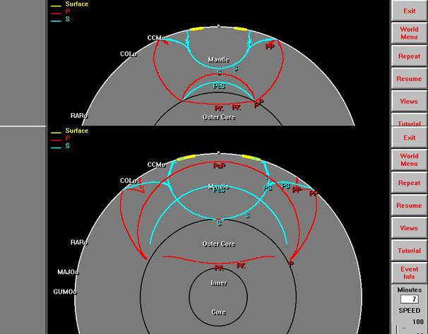
Figure 29. Partial
screen views of the Seismic Waves computer program. The upper image shows
seismic wavefronts traveling through the Earth's interior five minutes after
the earthquake. The lower image shows the wavefronts 7 minutes after the
earthquake. P waves are shown in red; S waves are shown in blue; and
Surface waves are shown in yellow. Three and four letter labels on the
Earth's surface show relative locations of seismograph stations that recorded
seismic waves corresponding to the wavefront representations in the Seismic
Waves program.
![]()
The Slinky: The slinky was invented in 1943 and over 250 million of them have been sold. The history of the slinky, including its invention and the information about the company that manufactures the slinky, can be found at the discovery and slinkytoys internet addresses in the reference list. Slinkys (Figure 30), including the original metal slinky, the plastic slinky, slinky junior, several "designer" slinkys made from a variety of metals, and slinky toys can be found at the slinkytoys internet address listed in the reference list. Both the original metal slinky and plastic slinkys are usually available (for about $2) at discount department stores such as K-Mart, Wal-Mart and Target. A "long" slinky can be ordered, but can also be made by taping together two regular slinkys with small pieces of plastic electrical tape to make a double-length slinky. The original metal slinky is the most effective type of slinky for most of the wave propagation activities. A double-length slinky is useful for illustrating Love wave motion (and the concept of standing waves) on the floor. The plastic slinky does not propagate compressional or shear waves as efficiently as the metal slinky, but is useful for illustrating reflection and transmission of wave energy at a boundary between two elastic materials with different properties. For this demonstration, tape a metal slinky and a plastic slinky together by attaching the end coils with small pieces of plastic electrical tape.
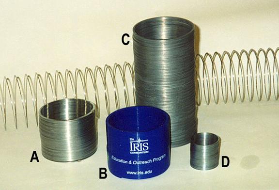
Figure 30. Slinkys. A. Original metal
slinky; B. Plastic slinky; C. Long slinky; D. Slinky junior.
Slinky lessons for teaching,
including physics and wave activities, can be found at the
Slinkys are educational and fun! It is useful to have many of them available for the activities described in this teachers guide and for your students to perform the activities, and to experiment and discover.
![]()
Summary: The slinky in various forms provides an excellent model to demonstrate and investigate seismic wave characteristics and propagation. A summary of the slinky models and their uses in demonstrations and activities is given in Table 3. Additional information on seismic waves, wave propagation, earthquakes and the interior of the Earth can be found in Bolt (1993, 1999 and 2004). Illustrations of seismic wave propagation through the Earth and seismograms are contained in Bolt (1993, 1999 and 2004) and Hennet and Braile (1998).
Table
3: Slinky Types, Models and Demonstrations
|
|||
|
Number |
Slinky Types/Models |
Demonstrations |
FigureNumber |
|
1 |
Regular metal slinky |
P and S waves |
13, 14 |
|
2 |
Long slinky (or attach 2 regular slinkys together with plastic electrical tape) |
Love wave on floor or tabletop |
--- |
|
3 |
Slinky with cardboard “building” |
Illustrate that P and S energy is propagating and causes the cardboard building to shake as wave arrives. Differences in shaking can be seen for P and S motion |
15, 16 |
|
4 |
Two slinkys (plastic and metal) attached with plastic electrical tape |
Reflection and transmission of energy at a boundary between materials of different types (elastic properties or seismic velocities) |
24, 25 |
|
5 |
Five slinkys attached to wood block |
Show that waves propagate in all directions from source; that travel time is different to different distances; and that wave vibration for P and S sources will be different in different directions from the source |
17,
18, |
|
6 |
Two slinkys attached to wood block, one with soft foam within the coils; cardboard buildings can be attached to the slinkys to help see the differences in shaking |
Illustrate the concept of attenuation due to absorption of energy during propagation and that some materials propagate waves more efficiently than other materials |
22, 23 |
![]()
Notes to the Teacher: The activities described in this teachers guide are designed for both classroom demonstration and inquiry-based activities for students. The elastic properties of a spring and the waves in a water tank activities are appropriate for student experiments. Several of the slinky activities and the human wave demonstration actively involve students in the class. The slinky demos should also be performed by the students to increase their understanding of the wave propagation characteristics and concepts. All of the activities provide opportunities for developing and practicing observation skills and experience with measuring and timing. These demonstrations and activities are suitable for inclusion in Earth science teaching at a variety of levels. At higher grade levels, more complete treatment, increased emphasis on necessary vocabulary (defining the properties of elasticity, describing the characteristics of motion of the different types of seismic waves, etc.), involving quantitative measurements (measuring and graphing the elasticity of a spring, calculating the velocity of propagation of waves, etc.), and connection to related seismology and other Earth science lessons and activities are desirable.
The depth of investigation and the length of time devoted to the seismic wave activities will depend on the grade level and characteristics of the students, time available, and teacher preference. The teacher will also need to determine the "degree of constructivism" to be employed in the teaching strategy for these demonstrations and activities. For example, several of the activities, such as the P- and S-wave propagation in a slinky, could be performed first as a demonstration and then by the students to develop further understanding by first-hand experience. Alternatively, the teacher could choose to have a brief classroom discussion about P and S waves and then challenge the students to use the slinky to discover P- and S-wave propagation and determine the primary characteristics of the waves (property of propagation, material returns to original condition after the wave has passed, reflection of wave energy, particle motion) and the distinctive differences between P and S waves. This student exploration would then be followed by a "final" demonstration to emphasize the key concepts and clarify any misunderstandings. The seismic wave activities should normally be included in an earthquake unit of an Earth science curriculum that also covers plate tectonics and the causes of earthquakes, Earth's interior structure, seismographs and seismograms, earthquake location methods, and earthquake hazards.
Appropriate assessment methods for the activities and science content presented here can include both written and oral responses by students and specific assessment activities. The scope and depth of questioning will depend on class level, time devoted to the seismic wave activities and how much related Earth science material (such as studies of plate tectonics, earthquake statistics and hazards, Earth structure, etc.) has been covered. If student teams have completed the elasticity of a spring, waves in water, and/or velocity of propagation experiments, the teacher will have some written material from the results of the student's experiments that can be assessed.
Here are some suggested activities that can be used for authentic assessment: (1) Have students perform the P and S wave slinky demonstrations and describe their observations and the wave characteristics that they observe. (2) Have students repeat the elasticity experiment with a spring that has a different spring constant (a "weaker" or "stronger" spring). Have students predict what the graphed line will look like in comparison with their previous result, then perform the experiment and graph the results. Their predictions should be close to the actual results. (3) Ask students to predict what would happen if a rubber band was used instead of the spring in the elasticity experiment (they should describe the expected result in terms of the two main properties of elasticity). (4) Provide the students with a graph showing a hypothetical seismic wave. Have the students interpret the graph and identify principal wave characteristics (frequency, amplitude, peaks, etc.). (5) Provide the students with copies of unlabeled diagrams illustrating the four types of seismic waves (lower three grids of the perspective views of P, S, Rayleigh and Love wave propagation in Figures 9-12 or from Bolt (1993, p. 27 and p. 37; remove labels identifying wave type). Have the students identify which diagram corresponds to the four types of seismic waves and what characteristics of the wave motion allow them to identify the wave type. (6) Obtain the Seismic Waves computer program and demonstrate to the students or provide the students with the opportunity to run the program. Next, with the program available on a monitor, start waves propagating (pause or restart as necessary) for one of the earthquakes and have the students watch the wavefront diagram (interior of Earth; it is convenient to set the display to view only the Earth cross section view; use the "Options" menu and "Select View …" to choose the cross section view) and have them answer the following questions. What are the approximate shapes of the initial (in the upper mantle near the source) P and S wavefronts? Why are they shaped that way? From the P and S wavefronts, estimate the relative velocity of the S wave as compared to the P wave (for example, how much longer does it take for the S wave to arrive at a station or to travel from the source to the core-mantle boundary as compared to the P wave)? How long does it take for the P wave to travel directly through the Earth to the opposite side of the Earth from the source? This distance (the diameter of the Earth) is about 12,742 km. From these measurements, what is the approximate average velocity for P waves in the Earth (in km/s)? Explain the new wavefronts that are generated when the P or S wave hits the core-mantle boundary. Why is there no S wave that travels directly through the Earth to the other side? Can there be S waves in the inner core (the program may not be of much help here except to visualize wavefronts that propagate in the Earth's core because no S wave phases from the inner core are displayed; not all seismic phases or raypaths are illustrated by the program)? How could S waves be generated so that they would travel through the inner core? Open the whole Earth view (surface of Earth with oceans and continents is visible). How are the patterns of the wavefronts that you see propagating and expanding from the source similar to the water waves in the wave tank experiment (or generated by a pebble dropped into a mud puddle or a pond)? How are they different?
Below are some suggested questions for a written assessment. (1) What is the source of energy for the generation of seismic waves; in the slinky demonstrations? in the Earth? (2) How could we demonstrate that energy is carried by the waves in the slinky demonstrations? (3) How can we determine the velocity of propagation of a wave? (4) Explain the property of elasticity. (5) Explain how the slow motions of the Earth's plates (like slowly deforming the stretched slinky in the P and S demonstrations alternative methods of wave generation) can produce a rapid release of energy (slip along a fault in an earthquake, release of stored elastic energy in the slinky) resulting in seismic waves propagating in the Earth (or the slinky).
![]()
NSES Standards: The activities and the science content contained in this teachers guide have significant connections to the National Science Education Standards (NSES; National Research Council, 1996; http://www.nap.edu/readingroom/books/nses/html/) as detailed in Table 4.
Additional related activities can be found at: http://web.ics.purdue.edu/~braile/. A simplified, four page version of this document can be found at: http://web.ics.purdue.edu/~braile/edumod/slinky/slinky4.htm. MS Word and pdf versions of these materials (easier for printing) can be found at:
http://web.ics.purdue.edu/~braile/edumod/slinky/slinky.doc
http://web.ics.purdue.edu/~braile/edumod/slinky/slinky.pdf
http://web.ics.purdue.edu/~braile/edumod/slinky/slinky4.doc
http://web.ics.purdue.edu/~braile/edumod/slinky/slinky4.pdf.
|
Table
4. "Seismic Waves and the Slinky: A Guide for Teachers" and
the National Science Education Standards (NSES; http://www.nap.edu/readingroom/books/nses/html/). |
|
NSES Standard
|
How standard is addressed by Seismic Waves and the
Slinky demonstrations, lessons and activities* |
Science Teaching Standards
|
Many of the activities
are inquiry-based (A, B) and provide opportunities for ongoing assessment
(C). |
Professional Development Standards
|
The guide for teachers
provides opportunities and appropriate resource material for teachers to
learn about an Earth science topic that is not likely to have been included
in their previous educational experiences (A, C) and includes suggestions for
effective teaching strategies (B). |
|
Assessment Standards |
Authentic assessment
activities and questions for assessing achievement in learning key concepts
are included (C). |
Science Content Standards
|
|
|
- Unifying Concepts and Processes in
Science |
Activities
provide experience with observation, evidence and explanation, and constancy,
change and measurement. |
|
- Science as Inquiry |
Activities
provide opportunities for practice of inquiry and of fundamental science
skills (Grades 5-8 and 9-12, A). |
|
- Physical Science Standards |
Activities
explore properties and changes of properties in matter, motion and forces,
transfer of energy (Grades 5-8, B). Activities
explore structure and properties of matter, motions and forces, and
interactions of energy and matter (Grades 9-12, B). |
|
- Earth and Space Science |
Activities
explore structure of the Earth system (Grades 5-8, D). Activities
relate to energy in the Earth system (Grades 9-12, D). |
|
- Science in Personal and Social
Perspectives |
Activities
explore natural hazards (Grades 5-8, F). Activities explore
natural and human-induced hazards (Grades 9-12, F). |
|
Table 4. (continued) |
|
|
Science Education Program Standards |
Seismic wave
activities are developmentally appropriate, interesting and relevant, and
emphasize student understanding through inquiry, and are connected to other
school subjects (B). Seismic wave activities provide practice with mathematics and analysis skills (C). Activities provide experience with a variety of materials and resources for experimentation and direct investigation of phenomena (D). |
|
Science Education System Standards |
Because only relatively simple and inexpensive resources are necessary to perform the seismic wave demonstrations and activities, they are easily accessible to all students. |
*Letters in parentheses identify specific standards within the six areas (Science Teaching, Professional Development, Assessment, Science Content, Science Education Programs, and Science Education System Standards) of the NSES.
![]()
Bolt,
B.A., Earthquakes and Geological Discovery, Scientific American Library,
W.H.
Bolt,
B.A., Earthquakes, (4th edition), W.H. Freeman & Company,
Bolt,
B.A., Earthquakes, (5th
edition; similar material is included in earlier editions), W.H. Freeman &
Company,
Earthquake, NOVA series videotape, 58 minutes, available from 800-255-9424; http://www.pbs.org, 1990.
Hennet, C., and L.W. Braile, Exploring the Earth Using Seismology – Color Poster, The IRIS Consortium, Washington, DC., www.iris.edu, 1998.
IRIS website, http://www.iris.edu.
Jones, Alan, Seismic Waves, Computer program for visualizing seismic wave propagation through the Earth's interior, download from: http://bingweb.binghamton.edu/~ajones/.
Living with Violent Earth: We Live on Somewhat Shaky Ground, Assignment Discovery series videotape, Discovery Channel, 25 minutes, http://www.dsc.discovery.com, 1989.
National Research
Council, National Science Education Standards, National
Rutherford, B.,
and S. A. Bachmeyer, Earthquake Engineering – The Epicenter Project Book,
Pitsco, Inc.,
Seismology – Resources for Teachers, http://web.ics.purdue.edu/~braile/edumod/seisres/seisresweb.htm, a list of seismology-related reference materials for education.
Shearer, P. M., Introduction
to Seismology,
Slinky websites:
http://www.discovery.com/stories/history/toys/SLINKY/shoulda.html
http://www.slinkytoys.com/main.htm
http://www.tpt.org/newtons/9/slink.html
http://www.teachingtools.com/SlinkyShindig/slinky.html
http://www.eecs.umich.edu/~coalitn/sciedoutreach/funexperiments/quickndirty/eweek/slinky.html
http://www.eweek.org/1999/Forms/disce.html#slinky
Zubrowski, B., Making
Waves, Beech Tree Books,
![]()
ãCopyright 2000-2010. L. Braile. Permission granted for reproduction for non-commercial uses.