|
Seismic Wave Demonstrations and Animations 1 L. Braile, braile@purdue.edu, web.ics.purdue.edu/~braile
|
December,
2004 (updated February, 2010)
|


Contents (click on topic to go directly to that
section; use the red up arrows to return to the list of contents):
4. P, S, Rayleigh and Love wave animations
6. Seismic Waves on Seismograms and Particle Motion Diagrams
8. Connections to National Science Education Standards (National Research Council, 1996)
[1]  Last modified February 26,
2010
Last modified February 26,
2010
The web page for
this document is:
http://web.ics.purdue.edu/~braile/edumod/waves/WaveDemo.htm
Partial funding for this development provided by the National Science Foundation.
ã Copyright 2004-10. L. Braile. Permission granted for reproduction and use of files and animations for non-commercial uses.
1. Introduction: Seismic wave animations are used to illustrate different types of wave propagation through elastic materials. Animations are provided to view wave propagation in a 3-dimensional solid for Compressional (P), Shear (S), Rayleigh (R) and Love (L) waves. Wave characteristics and particle motions of these wave types can be easily illustrated using the seismic wave animations.
This tutorial is available for viewing with a browser (html file) and for downloading as an MS Word document or PDF file at the following locations:
http://web.ics.purdue.edu/~braile/edumod/waves/WaveDemo.htm
http://web.ics.purdue.edu/~braile/edumod/waves/WaveDemo.doc
http://web.ics.purdue.edu/~braile/edumod/waves/WaveDemo.pdf
A related PowerPoint presentation for
seismic waves and the slinky is available for download at: http://web.ics.purdue.edu/~braile/new/SeismicWaves.ppt.
![]()
Return to list of contents
2. Seismic Waves: The main seismic wave types are Compressional (P), Shear (S), Rayleigh (R) and Love (L) waves. P and S waves are often called body waves because they propagate outward in all directions from a source (such as an earthquake) and travel through the interior of the Earth. In the animations shown here, the P and S waves are shown propagating horizontally, parallel to the Earth’s surface. Love and Rayleigh waves are surface waves and propagate approximately parallel to the Earth’s surface. Although surface wave motion penetrates to significant depth in the Earth, these types of waves do not propagate directly through the Earth’s interior. Descriptions of wave characteristics and particle motions for the four wave types are given in Table 1.
Further information on seismic waves, wave propagation in the Earth, and visualizations of seismic waves can be found in Bolt (1993, p. 27 and 37; 2004, p. 21) and Shearer (1999, p. 32 and 152). Information on teaching about seismic waves and demonstrations of seismic wave characteristics using a slinky are provided at:
http://web.ics.purdue.edu/~braile/edumod/slinky/slinky.htm. A four-page teacher’s guide about seismic waves and the slinky is available as an MS Word document at:
http://web.ics.purdue.edu/~braile/edumod/slinky/slinky4.doc,
or, as an html file at: http://web.ics.purdue.edu/~braile/edumod/slinky/slinky4.htm.
Table 1: Seismic Waves
|
|||
|
Wave Type (and names) |
Particle Motion |
Typical Velocity |
Other Characteristics |
|
P, Compressional, Primary, Longitudinal |
Alternating
compressions (“pushes”) and dilations (“pulls”) which are directed in the
same direction as the wave is propagating (along the ray path); and
therefore, perpendicular to the wavefront. |
VP
~ 5 – 7 km/s in typical Earth’s crust; >~ 8 km/s in Earth’s mantle and
core; ~1.5 km/s in water; ~0.3 km/s in air. |
P
motion travels fastest in materials, so the P-wave is the first-arriving
energy on a seismogram. Generally smaller and higher frequency than the
S and Surface-waves. P waves in a liquid or gas are pressure waves, including
sound waves. |
|
S,
Shear, Secondary, Transverse |
Alternating
transverse motions (perpendicular to the direction of propagation, and the ray
path); commonly approximately polarized such that particle motion is in
vertical or horizontal planes. |
VS
~ 3 – 4 km/s in typical Earth’s crust;
>~ 4.5 km/s in Earth’s mantle; ~ 2.5-3.0
km/s in (solid) inner core. |
S-waves
do not travel through fluids, so do not exist in Earth’s outer core (inferred
to be primarily liquid iron) or in air or water or molten rock (magma).
S waves travel slower than P waves in a solid and, therefore, arrive after
the P wave. |
|
L,
Love, Surface waves, Long waves |
Transverse
horizontal motion, perpendicular to the direction of propagation and generally
parallel to the Earth’s surface. |
VL
~ 2.0 - 4.4 km/s in the Earth depending on frequency of the
propagating wave, and therefore the depth of penetration of the waves. In general, the Love waves travel slightly
faster than the Rayleigh waves. |
Love
waves exist because of the Earth’s surface. They are largest at the
surface and decrease in amplitude with depth. Love waves are
dispersive, that is, the wave velocity is dependent on frequency, generally with
low frequencies propagating at higher velocity. Depth of penetration of
the Love waves is also dependent on frequency, with lower frequencies
penetrating to greater depth. |
|
R,
Rayleigh, Surface waves, Long
waves, Ground roll |
Motion
is both in the direction of propagation and perpendicular (in a vertical
plane), and “phased” so that the motion is generally elliptical –
either prograde or retrograde. |
VR
~ 2.0 - 4.2 km/s in the Earth depending on frequency of the
propagating wave, and therefore the depth of penetration of the waves. |
Rayleigh
waves are also dispersive and the amplitudes generally decrease with depth in
the Earth. Appearance and particle motion are similar to water waves. Depth of penetration of the Rayleigh waves
is also dependent on frequency, with lower frequencies penetrating to greater
depth. |
![]()
3. Seismic Wave Animations: Seismic wave animations for the P, S, Rayleigh and Love waves have been created using a 3-D grid shown in Figure 1. All wave types are designed to propagate in the X direction (illustrated in Figure 1) and parallel to the Earth’s surface. The wave animations illustrate wave characteristics and particle motion as listed in Table 1. However, no decrease in energy or amplitude with distance due to spreading out of the wave energy (geometrical spreading) or loss of amplitude caused by absorption of energy (sometimes called attenuation) by the media (due to anelasticity) are included. The elastic material is also assumed to be isotropic (velocity and other physical properties are the same for all directions of propagation), therefore, no anisotropy is included in the animations. Furthermore, for the surface wave animations, no dispersion (variation in wave velocity with frequency) has been included. The seismic wave animations were created using a Matlab code and then converted to an animated GIF format.
Other animations of P and S waves are contained in the Nova video "Earthquake" (1990; about 13 minutes into the program), of P, S, Rayleigh and Love waves in the Discovery Channel video "Living with Violent Earth: We Live on Somewhat Shaky Ground" (1989, about 3 minutes into the program) and in the 2003 Encyclopedia Britannica CD, Deluxe Edition (search for seismic waves), and of P (Longitudinal), S (Transverse), and Rayleigh waves at Prof. Daniel Russell’s website:
http://paws.kettering.edu/~drussell/demos.html. Wave propagation in the Earth can also be illustrated effectively using the simulation software Seismic Waves (developed by Alan Jones of SUNY, Binghamton) available at: http://bingweb.binghamton.edu/~ajones/.
|
|
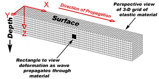
Figure 1. View of 3-D grid used
to illustrate seismic wave propagation.
The mesh (grid) represents a volume of elastic material through which
waves can propagate in the direction shown.
The 3-D grid is shown in perspective view to demonstrate the wave
propagation effects and particle motions of the different wave types in all
directions. In the animations shown
below, Compressional, Shear, Rayleigh and Love wave propagation through the
elastic material is illustrated. In this
3-D volume, the grid is designed to have an upper surface (corresponding to the
Earth’s surface) that consists of a boundary with a vacuum or very low density
fluid above so that surface wave propagation (Rayleigh and Love waves) as well
as body wave propagation (Compressional and Shear waves) can be illustrated.
![]()
4. P, S, Rayleigh and Love wave animations: Seismic wave animations (animated gifs that are viewed as html files using a browser such Internet Explorer or Netscape) can be opened by clicking on the images shown in Figures 2-5 below (use the Back or back arrow button in your browser to return to the current document).
P Wave Animation: Click on the image shown in Figure 2 to view the P wave animation. Notice the following wave characteristics and particle motion of the P wave:
The deformation (a temporary elastic
disturbance) propagates. Particle motion
consists of alternating compression and dilation (extension). Particle motion is parallel to the direction
of propagation (longitudinal). Material
returns to its original shape after the wave passes.
ã Copyright 2004-10.
L. Braile. Permission granted for
reproduction and use of animations for non-commercial uses.
Figure 2. Click on Figure to view Compressional (P) wave animation; use the Back button to return to the current document. To better understand the particle motion and characteristics of the P wave, notice the deformation of the black rectangle as the wave propagates through it.
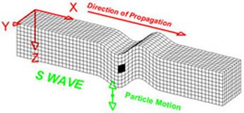
S Wave Animation: Click on the image shown in Figure 3 to view the S wave animation. Notice the following wave characteristics and particle motion of the S wave:
The deformation (a temporary elastic
disturbance) propagates. Particle motion
consists of alternating transverse motion.
Particle motion is perpendicular to the direction of propagation
(transverse). The transverse particle
motion shown here is vertical but can be in any direction; however the Earth’s approximately
horizontal layers tend to cause mostly SV (in the vertical plane) or horizontal
(SH) shear motions. Material returns to
its original shape after the wave passes.
ã Copyright 2004-10.
L. Braile. Permission granted for
reproduction and use of animations for non-commercial uses.
Figure 3. Click on Figure to view Shear (S) wave animation; use the Back button to return to the current document. To better understand the particle motion and characteristics of the S wave, notice the deformation of the black rectangle as the wave propagates through it.
Rayleigh Wave Animation: Click on the image shown in Figure 4 to view the Rayleigh wave animation. Notice the following wave characteristics and particle motion of the Rayleigh wave:
The deformation (a temporary elastic
disturbance) propagates. Particle motion
consists of elliptical motions (generally retrograde elliptical as shown in the
figure) in the vertical plane and parallel to the direction of
propagation. Amplitude decreases with
depth. Material returns to its original
shape after the wave passes.
ã Copyright 2004-10.
L. Braile. Permission granted for
reproduction and use of animations for non-commercial uses.
Figure 4. Click on Figure to view Rayleigh (R) wave animation; use the Back button to return to the current document. To better understand the particle motion and characteristics of the Rayleigh wave, notice the deformation of the black rectangle as the wave propagates through it. Also, if you focus on the top edge of the end of the 3-D grid while the wave is passing through that region, the retrograde elliptical particle motion is very clearly seen.
Love Wave Animation: Click on the image shown in Figure 5 to view the Love wave animation. Notice the following wave characteristics and particle motion of the Love wave:
The deformation propagates. Particle motion consists of alternating
transverse motions. Particle motion is
horizontal and perpendicular to the direction of propagation (transverse). To best view the horizontal particle motion,
focus on the Y axis (red line) as the wave propagates through it. Amplitude decreases with depth. Material returns to its original shape after the
wave passes.
ã Copyright 2004-10.
L. Braile. Permission granted for
reproduction and use of animations for non-commercial uses.
Figure 5. Click on Figure to view Love (L) wave animation; use the Back button to return to the current document. To better understand the particle motion and characteristics of the Love wave, notice the deformation of the black rectangle as the wave propagates through it. While viewing the Love wave animation, remember that the particle motion is purely horizontal (in the plus and minus Y direction in the diagram) and perpendicular to the direction of motion (the X direction in the diagram). Although it may appear in the animation (due to the perspective view of the 3-D grid) that the top surface of the grid is moving vertically (parallel to the Z axis), the particle motion is purely horizontal. To aid in seeing that the particle motion is horizontal and perpendicular to the direction of propagation, focus on the Y axis (red line) while the wave in the animations is propagating through the grid.
![]()
5. Downloads: The MS Word file for this document, individual animated html and gif files, and a PowerPoint presentation that includes the seismic wave animations, can be downloaded using the links listed below:
Download Seismic Wave Animated gif file as individual html files: After opening the animated gifs as html files by clicking on one of the figures (Figures 2-5) above, open the File menu and select the Save As option and save the animation as an html file.
Download Seismic Wave Animated gif files: Pwave Swave Rwave Lwave
(To view files, click on the file names [to view in browser], or right click on the file name, select Open With, and select Windows Picture and Fax Viewer. To download the files to your computer, right click on the file name and select Save Target As… [Internet Explorer] or Save Link As…[Firefox]. To view the downloaded files on your computer, right click on the file name, select Open With, and select Windows Picture and Fax Viewer.)
Download Seismic Wave
Demonstrations and Animations PowerPoint File: WaveDemo.ppt
Download Seismic Wave Demonstrations and Animations MS Word file: WaveDemo.doc
Download Seismic Wave Demonstrations and Animations PowerPoint File, continuous loop through the animations for the 4 wave types: WaveDemo4Types.ppt
Download Seismic Wave Presentation PowerPoint File: SeismicWaves.ppt
![]()
6. Seismic
Waves on Seismograms and Particle Motion Diagrams: The wave motion for actual earthquake
motions, as recorded on 3-component seismograms, can be compared with the
theoretical wave motion for the various wave types that are illustrated in the
seismic wave animations shown above.
Earthquake seismograms were examined for an M6.5 earthquake near the
west coast of
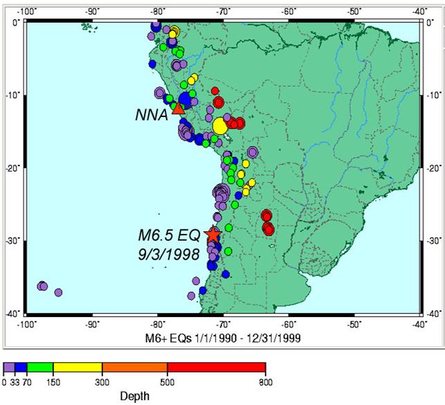
Figure 6. Location map and
historical seismicity in west central
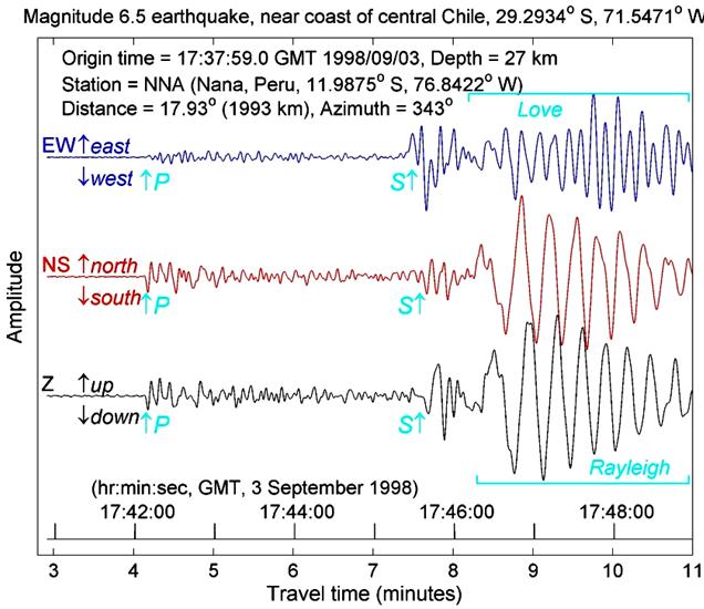
Figure 7. Seismograms
recorded by a 3-component seismograph at
Figure 8. Partial cross section
of the Earth showing major layer boundaries, approximate P-wave seismic
velocities (Vp), and approximate ray path for P- and S-waves from a shallow
earthquake to a seismograph at about 18 degrees (~2000 km) distance.
The seismograms in Figure 7 can also be shown as particle motion plots (two dimensional plots of the ground motion illustrating the motion in one plane) for specific phases (short segments of the records) as illustrated in Figure 9 for the seismograms in Figure 7. A 3-D perspective plot of the P-wave particle motion is also shown in Figure 10. For example, one can observe that the first motion of the P wave was down and to the south (see the Z and NS seismograms in Figure 7 and the upper left particle motion diagram in Figure 9). Note that the wave was traveling approximately from south to north from the epicenter to the NNA seismograph station (Figure 6). So, the Z-NS particle motion diagram (upper left hand corner of Figure 9) shows that the P-wave arrival (a longitudinal wave as illustrated in the animations described above) is arriving at an angle and from the south and the motion is down to the south and then up to the north (along the direction of the ray path which is diagonally from the lower left hand corner of the diagram). The EW-NS particle motion diagram (upper right diagram in Figure 9) shows the horizontal motion of the first arriving P wave and confirms that the motion is in the north-south direction with the first motion (small numbers on the particle motion line) to the south.
The first shear wave motion (illustrated in the particle motion diagram in the lower left of Figure 9) is arriving from down and to the south (diagonally from the lower left in the particle motion diagram). Although the shear wave motion is more complicated than the P-wave motion, the particle motion diagram shows that the motion is generally perpendicular to the direction of propagation, as expected from theory.
The Rayleigh wave particle motion plot is shown in the Z-NS plane in the diagram in the lower right of Figure 9. The Rayleigh wave from the earthquake propagated horizontally and almost directly from the south (from the left in the particle motion diagram in Figure 9). Following the numbers (which are spaced at 10 seconds apart on the seismogram), beginning with the number one, on the particle motion diagram, one can see that the Rayleigh wave particle motion is approximately retrograde elliptical (consistent with theory and the Rayleigh wave animation described above) and that a complete cycle is defined in about 20 seconds (note that the 4 and 6 labels and the 5 and 7 labels are nearly at the same location. One can also observe on the Z and NS seismograms (Figure 7) that the Rayleigh wave energy, in the area of the seismogram corresponding to the maximum amplitudes, is of approximately 20 s period.
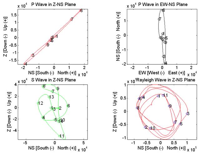
Figure 9. Particle
motion diagrams for selected seismic waves from the seismograms shown in Figure
7. Plots illustrate the particle motion
by plotting seismograms for two components of motion, one component on the
horizontal axis and one component on the vertical axis (two horizontal
components for the diagram in the upper right).
The relative amplitude of ground motion in each direction is indicated
by the axis labels. Numbered circles on
the particle motion plots show successive times (every 1 second beginning at
17:42:07 UTC/GMT time for the P wave particle motion plots – 8 s record; every
2 seconds beginning at 17:45:33 UTC/GMT time for the S wave particle motion
plot – 26 s record; and every 10 seconds beginning at 17:46:30 UTC/GMT time for
the Rayleigh wave particle motion plots – 100 s record). P-wave particle motion is shown for the Z-NS
plane (upper left graph) and for the EW-NS plane (upper right graph. S-wave particle motion is shown for the Z-NS
plane in the graph at the lower left.
Rayleigh-wave particle motion is shown for the Z-NS plane in the graph
at the lower right.
Because the Love wave motion is
purely horizontal and the NNA station is almost directly north of the
epicenter, the particle motion on the east-west component seismogram after
about
Finally, a 3-D view of the P wave particle motion is illustrated in Figure 10. The bold arrow shows that approximate direction of approach of the P wave energy at the NNA seismograph, corresponding to a ray path coming up and from the south (similar to the ray path shown in Figure 8).
Figure 10. Particle
motion diagram for the P wave from the seismograms shown in Figure 7. Three-D perspective plot illustrates the
particle motion by plotting seismograms for three components of motion, two
components on the horizontal axes and one component on the vertical axis. The relative amplitude of ground motion in
each direction is indicated by the axis labels. Numbered circles on the particle motion plot
show successive times (every 1 second beginning at
![]()
7. Teaching Strategies: We provide the following suggestions and activities for using the seismic wave animations and other materials in this document for educational purposes.
1. We suggest that demonstration and discussion of the seismic wave animations be preceded or followed by some of the slinky demonstrations and activities (Seismic waves and the Slinky: A Teachers Guide,
http://web.ics.purdue.edu/~braile/edumod/slinky/slinky.htm,
or the four page slinky document,
http://web.ics.purdue.edu/~braile/edumod/slinky/slinky4.doc). The slinky demonstrations can be used to reinforce and extend the understanding of seismic wave types and seismic wave propagation and provide hands-on, discovery experiences with waves.
2. The seismic wave animations can be used to introduce the four seismic wave types and the particle motion characteristics of the wave types. View the wave animations several times and review the characteristics of each wave type. (The html version of the seismic waves demonstrations and animations or the PowerPoint presentation – see downloads above – are convenient methods for viewing and discussing the demonstrations and animations.) Focusing on one area of the 3-D grid such as the black rectangle or the top edge at the end of the grid is an effective method for observing the particle motion characteristics. Use the un-labeled seismic wave types diagrams (Figure 11) to quiz the class on recognizing the characteristics of the waves and particle motions.
What
seismic wave type is shown here?
|
|
|
|
|
|
Figure 11.
Click on the question above to view (link to an html file) un-labeled
diagrams of the four seismic wave types to use as a quiz. (Use the Back
or back arrow button in your browser to return to the current document.)
3. The second half of the seismic wave animations document (this document, section 6) compares the seismic wave animations with actual seismograms, seismic waves from an earthquake source, and particle motion diagrams derived from the 3-component seismograms. Although the details of the seismograms and the particle motion diagrams are complicated and visualization of the 3-D nature of the wave motion is somewhat difficult, the primary objective of this section is to show that real seismic waves are consistent with the theoretical features of the wave animations. Depending on the experience level of your audience and the amount of time that you wish to devote to study of seismic waves, use of the seismogram and particle motion material may be limited.
4. Observation of the seismic wave demonstrations and animations can be followed by use of the Seismic Wave computer program to view simulations of seismic waves propagating through a spherical Earth model. Wave types, refraction and reflection of seismic waves, Earth structure and wave propagation characteristics can be studied using the Seismic Waves software (available at: http://bingweb.binghamton.edu/~ajones/). It should be noted that seismic wave propagation in the Seismic Waves program is simulated by viewing wave fronts instead of following wave energy along the direction of propagation (ray paths). Wave fronts and ray paths are described and illustrated in the slinky guide. Some teaching strategies for use of the Seismic Waves software are also provided in the slinky guide,
http://web.ics.purdue.edu/~braile/edumod/slinky/slinky.htm.
5. The 3-component seismograms illustrated in Figure 7, above, can be downloaded here (in SAC format; NNA.BHZ.sac, NNA.BHN.sac, NNA.BHE.sac) and plotted using the AmaSeis software. An effective method to view the seismograms and observe the characteristics of the waves as they arrive at the seismograph station is to display the three seismograms on the AmaSeis screen (by opening the SAC files; hold down the control key, Ctrl, to select all three files for opening in one AmaSeis display window) and use the Play record feature to play back the seismograms in speeded up time (a speed scale factor of about 8 is effective). Instructions for downloading and installing the AmaSeis software and using the play back features described here are available at:
http://web.ics.purdue.edu/~braile/edumod/as1lessons/UsingAmaSeis/UsingAmaSeis.htm (see sections 3.8 and 5.4).
6. Simulations of the seismic wave types and wave motion can be performed by your students using the following method. Cut several 35-40 cm diameter circles out of poster board or cardboard. Have students who are going to demonstrate seismic waves hold the circular pieces in front of them with both hands as shown in Figure 12. The particle motion for each wave type is illustrated in the diagrams in Figure 12. Have the students move the circular pieces as shown while walking forward to simulate wave propagation and the particle motion of a specific wave type. Note that the S wave is shown with vertical (up and down) transverse motion (Figure 12) although the transverse motion could be horizontal or in any direction perpendicular to the direction of propagation. Using the vertical transverse motion for the S wave helps distinguish it from the Love wave. Also, the diagram for the Love wave (Figure 12) may appear to show diagonal motion (it is a perspective view), whereas the Love wave motion is horizontal and perpendicular to the direction of propagation. Use the following activities to demonstrate aspects of the seismic wave types and seismic wave propagation:
a. Single wave type demonstration: For each wave type, have one or more students perform the propagation and particle motion simulation. Do the simulation for one wave type at a time. Compare the simulation with the seismic wave animations. Follow up by having one or more students perform one of the wave type simulations without announcing to the class which wave type was selected. While the students are demonstrating the wave type, ask students in the class to identify the seismic wave and the properties that characterize it. What characteristics of the wave cannot be represented by the simulation (compare with the animations and the properties listed in Table 1)?
b. Waves in all directions demonstration: Have 4-6 students with the circular pieces stand in the center of a room facing outward in different directions. At your signal, have the students walk away from the central location (in all directions) and perform one of the wave simulations. Do the simulation for one wave type at a time. This activity demonstrates that the various wave types propagate from a source location (such as the focus of an earthquake) in all directions (the surface waves always propagate approximately parallel to the Earth’s surface). What characteristics of wave propagation cannot be represented by the simulation (compare with the animations and the properties listed in Table 1)?
c. Four wave types propagating at once demonstration: Have four students with circular pieces stand in a line at one side of the room facing away from the wall. At your signal, the students all walk forward performing a wave motion simulation. The first student walks fast and demonstrates the P-wave motion. The second student walks at a medium speed and demonstrates the S-wave motion. The last two students walk slowly and one demonstrates the Rayleigh wave motion and the other demonstrates the Love wave motion. This activity shows that all four wave types propagate, and that they travel at different speeds and have relatively distinct motion. What characteristics of wave propagation cannot be represented by the simulation (compare with the animations and the properties listed in Table 1)? With twelve or sixteen students, one can simulate the four wave types and different speeds and have the waves also propagate in different directions at the same time illustrating wave energy spreading out from a source.
In association with the seismic wave animations, the use of the slinky demonstrations, and other information and demonstrations related to waves, these activities can be effective tools for enhancing learning. The activities, particularly the simulations, allow hands-on experience and concrete modeling of wave phenomena that can improve understanding, reinforce fundamental concepts and theory, generate interest, and allow student discovery.
Figure 12. Schematic diagram
illustrating students performing wave simulations. Student holds a poster board or cardboard
circle in front of his or her body and walks forward (like the seismic waves
propagating in the Earth). While
walking, the student moves their circle forward
and backward (“push and pull”, for the P wave), or up and down (transverse motion for the shear wave), or in a retrograde ellipse (for the
Rayleigh wave), or side to side horizontally
(for the Love wave), as shown above.
![]()
8. Connections to National Science Education Standards (National Research Council, 1996): Seismic waves, wave propagation in the Earth and energy carried by seismic waves are related to the following science standards: Content Standards: Science as Inquiry – practice inquiry and fundamental science skills (grades 5-8 and 9-12, A); Physical Science – properties of matter, motion, transfer of energy (grades 5-8, B), structure of matter, motion, interactions of energy and matter (grades 9-12, B); Earth and Space Science – relate to energy in the Earth system (grades 9-12, D).
![]()
Bolt, B.A., Earthquakes and Geological Discovery, Scientific American Library,
W.H.
Bolt, B.A., Earthquakes, (5th edition; similar diagrams are included
in earlier editions of Earthquakes),
W.H. Freeman & Company,
Earthquake, NOVA series videotape, 58 minutes, available from 800-255-9424; http://www.pbs.org, 1990.
Encyclopedia Britannica, CD, Deluxe Edition, http://www.britannica.com/, 2003.
Living with Violent Earth: We Live on Somewhat Shaky Ground, Assignment Discovery series videotape, Discovery Channel, 25 minutes, http://www.dsc.discovery.com, 1989.
National Research Council, National
Science Education Standards, National
Shearer, P. M., Introduction to
Seismology,
![]()
10. Acknowledgements: Thanks to George Jiracek for suggesting the addition of the black rectangle on the seismic wave animation diagrams for better recognition of particle motion, and to Sheryl Braile for suggesting the hands-on seismic wave simulation activity described in activity number 6 in the Teaching Strategies section (section 7). Partial funding for this development provided by the National Science Foundation.
![]()