

EqLocate Tutorial 1
(L. Braile, July 2002, revised November,
2004)
http://web.ics.purdue.edu/~braile
About EqLocate: EqLocate
is an interactive earthquake location program that uses actual seismograms and
user-selected P-wave arrival times to locate the earthquake. The program uses a method that is similar to
the approach that is used by seismologists to routinely determine the location
of earthquakes from around the world. In
the standard method, tens to hundreds of arrival times (each from an individual
seismogram corresponding to a seismograph station) are used by a computer
program to automatically find an optimum solution (location and origin time of
the earthquake determined such that the observed arrival times match the
theoretical arrival times calculated using a well-known seismic velocity model
for the Earth). In EqLocate, a limited
number of seismograms (
Several data sets (seismograms) for selected earthquakes are provided with EqLocate. Additional data can be added to the EqLocate folder at any time. Although EqLocate can be used to locate many earthquakes, and the resulting locations are reasonably accurate, the primary objective of the program is to illustrate the important concepts of earthquake location for educational purposes.
The EqLocate program was written by Alan Jones based on a concept developed by Larry Braile. John Lahr and Larry Braile provided testing and suggestions during program development. Support for development of the program was provided by the NSF-sponsored IRIS (Incorporated Research Institutions for Seismology) Consortium.
Four sections of this tutorial (Running EqLocate, How EqLocate Works, Importing Data into EqLocate, and Data Sets) are provided below to explain the use of the program to locate earthquakes, to understand the method used by the program, and to learn about earthquake data (including importing data into EqLocate) and earthquake location.
List of Contents (click on topic to go directly to that section, use
the red up arrows to return to the List of Contents):
1.4 Opening seismograms from an earthquake folder
1.5 Finding the earthquake epicenter
1.6 Estimating the possible error in the derived epicenter
1.7 Determining the depth of focus of the earthquake
1.8 Checking the accuracy of the solution
2.2 Seismograms recorded at seismograph stations
2.3 Flow chart for the EqLocate program
2.4 An additional example of the use of EqLocate
3. Importing data into EqLocate
1. Running EqLocate: This section describes how to
install and operate the EqLocate program on your computer. EqLocate runs on the Windows operating
system.
1.1 Installing EqLocate: To install EqLocate on your computer, use your Netscape or Internet Explorer browser to link to: www.geol.binghamton.edu/faculty/jones/EqLocateSetup.exe. Download the file EqLocateSetup.exe to your computer (saving it in a folder called “Downloads” is convenient as you can reinstall at some later time or copy or send the file for another computer) and double click on EqLocateSetup.exe. The setup program will install EqLocate on your computer in a folder called EqLocate. In the EqLocate folder, right click on the EqLocate.exe file and create a shortcut to EqLocate.exe. Drag the shortcut to your desktop.
![]()
1.2 Starting EqLocate: To start EqLocate, double click on the EqLocate.exe shortcut on your desktop. A “splash screen” with information about the program will appear. Click continue. A world map similar to that shown in Figure 1 will appear. You can change the map view and zoom in using the arrow and plus and minus controls as illustrated in Figure 2. Zoom in on the map and adjust the view to the approximate area of the earthquake that you wish to view. You can select one of the standard earthquake data sets (seismograms located in folders organized by event) provided with the program or generate your own seismogram folder by downloading data from the IRIS Data Management Center using WILBER (see Importing Data Into EqLocate below) or other source of SAC binary seismogram files such as AS-1 or PEPP.
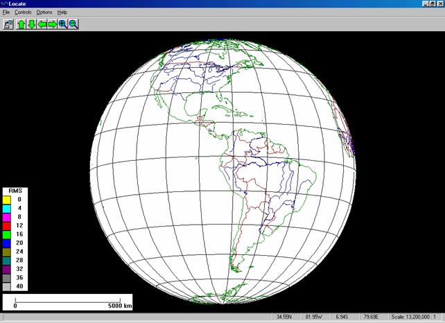
Figure 1.
Screen image of the EqLocate program showing world map display. Any area of the world can be displayed and
the user can zoom in to focus on the area that included the seismograph stations
of interest. Latitude and longitude
lines at 15 degree intervals are shown on the map.
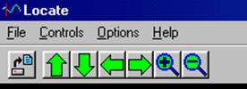
Figure 2. Close-up of the EqLocate controls for moving
around the world map and zooming. The up
arrow causes the world view to move to the north. The down arrow causes the world view to move
to the south. The left arrow causes the
world view to move to the west. The
right arrow causes the world view to move to the east. The plus symbol causes zooming in (smaller
area displayed) on the view. The minus
symbol causes zooming out (larger area displayed).
![]()
1.3 EqLocate menus: Pull-down menus in EqLocate (at the upper
left hand corner of the screen) provide controls and program information. Using the File menu, one can open or
close seismogram files for events, print the current screen, and exit the
program. In the Controls menu,
one can set the depth of focus (a dialog box appears that allows the user to
select from several standard depths or input an arbitrary depth – the travel
time tables are limited to a maximum depth of about 650 km because only a few
earthquakes deeper than that depth have ever been recorded) of an earthquake to
iteratively determine the depth as well as the epicenter; set the maximum RMS
value for the color coding on the color bar at the lower left hand corner of
the screen – for most regional and distant (teleseismic) events, a value of 30
or 40 works well; use the zoom and arrow controls equivalent to the arrow and
plus/minus symbols in the upper lest hand corner of the screen (Figure 2). In the Options menu, one can turn on
the Hints window that provides a shorter version of the instructions that are
provided here; select multiple seismogram windows (small windows displaying one
seismogram for each station that can be moved to be located adjacent to the
station location), or seismograms in one window. In the Help menu one can determine the
version of EqLocate that is installed and some information about the
program. During program operation, Hints windows appear that help guide
the user through program operation.
![]()
1.4 Opening seismograms from an earthquake
folder: To open seismograms
for an earthquake, select Open Event from the File menu and
select the event of interest. The
seismograms for each standard event are saved in a folder named for the
event. Open the folder by double
clicking or selecting and clicking on Open and select the seismograms
using the mouse. Hold the Control
key down to select multiple seismograms.
Hold the Shift key down and select the first seismogram
and the last seismogram to select all seismograms in the folder. Click Open. At least three seismograms should be selected
for each event.
New seismograms for additional
earthquakes can be added. Place
seismograms in folders to organize the data by event as has been done with the
standard earthquakes provided with EqLocate.
Occasionally, an opened seismogram will have an arrival time that cannot
be matched with a theoretical travel time.
In this case, it is possible that a timing error exists with that
seismogram and station and therefore, that seismogram should not be used for
locating the earthquake. For more
information on adding seismograms, see Importing Data Into EqLocate below.
An example of opening seismograms
for an event is shown in Figure 3. In
this example, the
One can also select multiple
seismogram windows (use the Options menu) in which case there will be
one window for each seismogram. The
seismogram windows can be moved around on the screen to place them adjacent to
the corresponding station. Time and
amplitude expansion of the traces is also provided by the arrows in each of the
multiple seismogram windows.
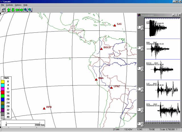
Figure 3. Screen image of the EqLocate program after an
earthquake data set (in this case the
With the single window view, as in Figure 3, one can
enlarge the seismograms window by dragging the lower left hand corner of the
window with the mouse cursor. The time
scale can then be expanded if desired and the amplitude of each trace can be
expanded as needed. Then, placing the
cursor at the interpreted first arrival (P-wave) of each seismogram, clicking
the mouse selects the arrival time (indicated by a red vertical line). The resulting display for the
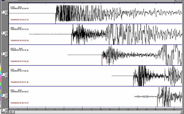
Figure
4. Screen image of the EqLocate program
seismogram window. The window has been
enlarged on the screen by dragging the lower left hand corner of the window to
the left. Also, the time scale has been
expanded by a factor of 2 using the up arrow in the lower left hand corner of
the seismogram window. Amplitude scales
of some of the seismograms have been enlarged (for easier interpretation of the
first arrival) using the up arrows located to the left of each seismogram. Arrival times for each seismogram have been
picked by clicking the mouse with the cursor positioned at the user-selected
arrival time. The selected arrival times
are marked by a red line extending downward from the seismograms. The scale at the bottom of the window is
relative time in minutes. To the left of
each seismogram is information about the station and seismogram. The station name is a 3, 4 or 5 letter
code. BHZ indicates the vertical
component of motion from a broadband seismograph. The second line of text lists the date
(YYYY/MO/DA) and the time of the start of the seismogram (HR:MN:SS.ss). The next line gives the date (YYYY/MO/DA) and
the arrival time (HR:MN:SS.ss).
![]()
1.5 Finding the earthquake epicenter: Next, the
initial trial epicenter is selected by clicking on the map display. In practice, any location will work to start
the process, but because we have seismograms that are all recorded and
displayed in absolute time, we know that the epicenter must be closest to the
station corresponding to the seismogram with the earliest travel time. Therefore, one should select an initial trial
epicenter near the station with the earliest arrival time. For the
The degree to which the data from the trial epicenters
fits the observed arrival times (“the quality of the solution”) can be
visualized and understood with three different but related displays. After the trial epicenter is selected, the
epicenter-to-station distances are calculated by the program and theoretical
travel times for each of these distances can be calculated by interpolation of
the standard travel time curves, and an origin time for the earthquake estimated. The theoretical arrival times are then
calculated and compared with the observed (user-selected, or, “picked”) arrival
times. A consistent measure of the fit
of all the arrival time data is the RMS
(Root Mean Square) error (the RMS error is a measure of the average
error of the observed minus theoretical arrival times) shown on the yellow bar
near the upper left hand corner of the map display. For the
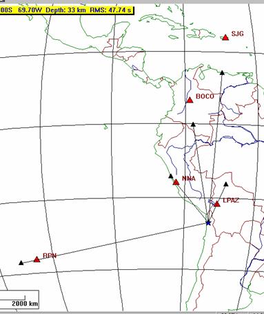
Figure 5. Portion of the
EqLocate screen after the initial trial epicenter (small blue star) has been
selected. A depth of 33 km was chosen
for the initial trial epicenter. The
small black triangles and lines extending from the trial epicenter toward the
stations indicate the estimated distance to each station based on the arrival
times and the origin time estimated from an average of the time information
(see How EqLocate Works, section
2, below). The black lines are simply straight lines
connecting the epicenter with the estimated epicenter-to-station distance (from
the observations – not the distance calculated from the coordinates of the
trial epicenter and the stations). These
lines do not represent the paths that the seismic waves would travel. The paths would be slightly curved lines on
this map projection connecting the trial epicenter and the station. The RMS error (in this case 47.74 s)
indicates that our trial epicenter is not a good solution. The fact that the calculated
epicenter-to-station distances (from epicenter to each station – red triangle)
do not match the estimated distances (epicenter to small black triangles) also
indicates that the initial epicenter is not correct. Comparing the observed and theoretical
arrival times in the seismogram window also confirms that the trial epicenter
is not correct.
Theoretical arrival times that are earlier than the observed arrival time indicate that the trial epicenter needs to be moved farther from that station. Similarly, theoretical arrival times that are later than the observed arrival time indicate that the trial epicenter needs to be moved closer to that station.
An additional
display of the fit of the trial epicenter and of the direction to move the
epicenter for a better fit is provided by the black triangles and lines on the
map display. The positions of the small
black triangles and the lengths of the lines are calculated by the program and
represent the expected distance to the corresponding station if the
trial epicenter is correct. A mismatch
in the positions of the triangles means that the trial epicenter needs to be
moved. If the estimated distance is less
than the epicenter-to-station distance (the line connecting the epicenter to
the small black triangle does not reach the station), the epicenter needs to be moved toward that station. Similarly, if the estimated distance is
greater than the epicenter-to-station distance (the line connecting the
epicenter to the small black triangle goes through the station), the epicenter needs to be moved farther
from that station. For example, for
the initial trial epicenter for the
An additional feature appears in the map display for the second trial epicenter (Figure 6). Because the RMS error is less than the maximum RMS error that we have set for the color bar on the map (in this case, 40 s; use the Controls menus to set the maximum RMS error for the color bar display), the second trial epicenter is color-coded, providing a quick, visual indication of the degree of fit of the location. However, in this case, the relatively high RMS error, the mismatch of the estimated and actual station locations, and the mismatch of the observed and theoretical arrival times (visible in the seismogram window) all indicate that the trial epicenter is still not good enough.
The search can
be continued by selecting another trial epicenter using the positions of the
small black triangles as guides to which direction to move the epicenter. A relatively small RMS error solution can usually be found with a few more trials
using this approach. However, a very
effective alternative, and one that provides additional insight into the
solution, is to simply try many epicenters near the location where a relatively
low RMS error solution has been
found. Because the program calculates
new solutions so rapidly, it is very fast and easy to search for the optimum
location using this method. For example,
for the
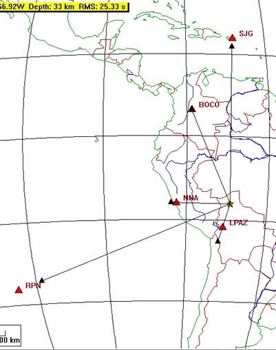
Figure 6. Portion of the
EqLocate screen after the second trial epicenter (small blue star) has been
selected. The location is improved – the
estimated epicenter-to-station distances derived from the arrival time data (small
black triangles connected to the epicenter by thin lines) are closer to the
theoretical distances (epicenter to station), and the RMS error has decreased
significantly.
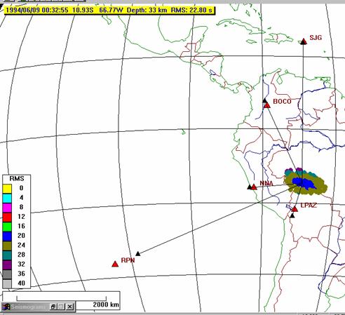
Figure 7. Portion of the
EqLocate screen after the best solution has been found for the initial depth of
focus – 33 km. The RMS error has been
reduced but it is still large. This
error corresponds to an average of many seconds of error per station, whereas
arrival time accuracy is about one second or less. The mismatch of the small black triangles and
the station locations also indicates that the solution is not very good. However, by selecting epicenters all around
the lowest RMS error epicenter, the RMS color pattern shows that this epicenter
is optimum for the chosen depth. This
pattern also provides an estimation of the uncertainty in the epicenter
location.
![]()
1.6 Estimating the possible error in the derived epicenter: For the depth of focus that was originally selected (33 km), the best solution found corresponded to an RMS error of 22.8 s (Figure 7). Furthermore, by selecting many trial epicenters, an approximately elliptical-shaped area has been outlined by the colors on the map. The colors show that the lowest RMS error epicenter is near the center of this ellipse and the size of the ellipse gives an indication of the possible error in the derived solution. For example, one can see that the central blue area (corresponding to an RMS error that is somewhat less than the solutions in the surrounding area) is about 600 km wide. Because any epicenter in the blue area has about the same RMS error (in this case, between 20 and 24 s), the different locations are not significantly different in the degree of fit to the observed data. Thus we might conclude that the accuracy of our epicenter is about +/- 300 km. A more complete estimation of the possible inaccuracy of the epicenter is somewhat more complicated and requires the knowledge (or reasonable assumption) of the accuracy of the data including the observed arrival time accuracy, the accuracy of the locations of the stations, and the validity of the Earth model that is used to calculate the travel time curves. However, color-coding of regions of error in the earthquake location, as shown in Figure 7, is at least a useful relative indicator of the accuracy of the solution.
![]()
1.7 Determining the depth of focus of the earthquake: The RMS error for the best solution shown in Figure 7 is still relatively large. More data (seismograms from additional stations) might help, but a likely problem that we have not addressed thus far is the depth of focus of this earthquake. The depth of 33 km was chosen arbitrarily as a starting depth because most earthquakes are relatively shallow. However, the large RMS error and the significant mismatch in the distances (as indicated by the triangles on the map in Figure 7) suggest that the depth of focus might be significantly different than 33 km. We can easily test this hypothesis by selecting other depths and then selecting new trial epicenters. Setting the depth is easily accomplished using the Depth window that is opened from the Control menu. Performing multiple epicenter searches as illustrated in Figure 7 for a variety of depths yields locations with RMS errors that are shown in Table 1. The errors decrease significantly for the optimum trial epicenters corresponding to greater depth of focus. The minimum RMS error is found for a depth of focus of 650 km although there is very little difference in the errors found for any depth from about 580 km to 650 km. The resulting solution is shown in Figure 8.
Table 1. Depth of focus and minimum RMS error for the
|
Depth of Focus
(km) |
Minimum RMS Error (s) |
|
33 |
22.8 |
|
100 |
21.1 |
|
200 |
18.9 |
|
300 |
14.5 |
|
400 |
9.3 |
|
500 |
6.7 |
|
600 |
1.8 |
|
650 |
1.7 |
The small RMS error, the comparison of the estimated and calculated distances to each station (correspondence of the small black triangles and the red triangles), and the match of the observed and theoretical arrival times in the seismogram window (Figure 9), all indicate that the epicenter shown in Figure 8 provides a very good fit to the observed arrival times. Furthermore, the small error ellipse (the yellow area outlined in Figure 8 representing epicenters corresponding to RMS errors of less than 4 s) suggests that the derived location is reasonably accurate (about +/- 50 km in epicenter location and +/- 70 km in depth).
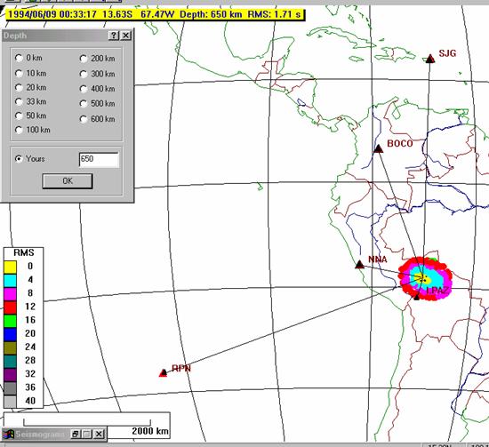
Figure
8. Portion of the EqLocate screen after
the final trial epicenter (small blue star) has been selected. Various depth of focus values were tried up
to 650 km (very few earthquakes have been recorded that have depths greater
than 650 km). The small RMS error (1.71
s), the match of the estimated distances and the theoretical distances (black
and red triangles are almost at the same location), the small error ellipse
defined by the colors, and the small observed minus theoretical arrival time
differences seen on the seismogram display, indicate that the earthquake
location (latitude, longitude, depth of focus and origin time) determined using
these seismograms and EqLocate is accurate.
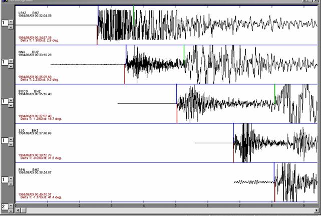
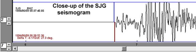
Figure 9. EqLocate seismogram
window (upper diagram) for the
![]()
1.8 Checking the accuracy of the solution: To check the accuracy of the location, a comparison between the “official” location and the location determined using the five seismograms and EqLocate is shown in Table 2. As can be seen from Table 2, the EqLocate solution is very good. The official location information for earthquakes can be found from the earthquake search tool on the US Geological Survey web page (http://earthquake.usgs.gov) or using the event search tool on the IRIS DMC web page (http://www.iris.edu). Detailed instructions (including examples) for accessing earthquake information from the Internet for recent and historical events are provided at:
http://web.ics.purdue.edu/~braile/edumod/eqdata/eqdata.htm (see section 2.3).
Table
2. Comparison of the official (USGS)
location (latitude, longitude, depth and origin time) for the Bolivia
earthquake determined from over a hundred arrival times, with the EqLocate
location determined from the five seismograms shown here.
|
|
Official Location
|
EqLocate Location
|
|
Latitude (degrees S) |
13.84 |
13.63 |
|
Longitude (degrees W) |
67.55 |
67.47 |
|
Depth of focus (km) |
631 |
650 |
|
Origin Time (HR:MN:SS, GMT/UTC) |
|
|
![]()
1.9 Selection of seismograms: In selecting seismograms to use in EqLocate to determine the epicenter or hypocenter of an earthquake, one should select at least 3 seismograms to obtain an estimate of the epicenter (there are 3 unknowns to determine – latitude, longitude and origin time) and at least 4 seismograms to obtain an estimate of the hypocenter (there are 4 unknowns to determine – latitude, longitude, origin time and depth of focus). Using additional seismograms (stations) will generally improve the accuracy of the solution. In practice, using about 5-8 seismograms will provide for a rapid and reasonably accurate solution. Selecting at least one station that is reasonably close to the epicenter (one usually knows the approximate location for significant events from damage or felt reports even before a calculated location is available, although calculated locations are sometimes available on the Internet just a few minutes after the earthquake), will improve the solution, especially for deep focus earthquakes. Also, the seismograph stations should approximately “surround” the epicenter, and especially not be all from the same direction. As an example of this problem, three seismograms were used to locate the Northridge earthquake using EqLocate (Figure 10). Because the stations selected and the epicenter are located approximately along a line, the resulting location is very poorly determined. The best fitting epicenter corresponds to a very low RMS error (0.39 s), but solutions (epicenters) that are almost as good are found in a very broad region outlined in Figure 10 by the color-coded RMS errors for many trial epicenters. The “banana” shape of this region is caused by the station locations with respect to the epicenter. Because the stations are located approximately along a line, the arrival time data for the three stations provide a very poor “triangularization” of the epicenter. For this set of stations, a small error in one of the observed arrival times (from “picking” the wrong arrival, from noise on the seismogram, or from timing errors in the seismograph station) could result in a fairly large error in the epicentral solution.
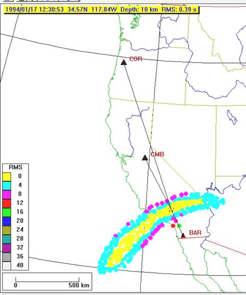
Figure 10. Color-coded RMS errors for trial epicenters
for the Northridge (January 17, 1994) earthquake using EqLocate and only three
seismograms. Epicenters corresponding to
solutions with RMS errors less than 4 s are indicated by the yellow area.
![]()
2. How EqLocate Works:
2.1 Monitoring earthquakes: Seismograph stations around the world continuously record seismic data (vibrations of the ground) to monitor earthquake activity and detect and record the signals from explosions. These seismographs also record seismic signals from various noise sources such as ocean waves hitting the coastline (a primary cause of microseisms), wind, nearby traffic, sonic booms, volcanic eruptions, lightning and thunder, and other sources of ground vibration. When a significant earthquake occurs, seismic waves travel through the Earth’s interior and the waves are recorded on seismographs around the world. A seismogram from a single seismograph station cannot be used to determine where the earthquake occurred. In fact, from the compressional or P-wave arrival time (the compressional wave is the earliest arrival and its time is usually accurately determined) recorded on a single seismogram, we cannot determine the location, distance or origin time of the event. If an S-wave is also identifiable on the seismogram, the distance from the station to the earthquake and the origin time can be estimated from the single station record using the difference in the time of arrival of the S- and P-waves. This difference is proportional to the distance from the station. If S- and P-wave arrival times are available from three or more stations, it is possible to determine the epicenter (with some accuracy) by triangulation using the S minus P times. This S minus P method is relatively easy to use and the method is instructive for learning about earthquake location and seismic waves. More information about earthquake location methods and the S minus P method can be found in Bolt (1993, p. xxx), and the following Internet sites:
http://quake.wr.usgs.gov/info/eqlocation/, http://www.scecdc.scec.org/Module/s3act03.html,
http://www.geo.mtu.edu/UPSeis/locating.html,
http://www.geol.vt.edu/outreach/vtso/anonftp/iasphand/CD_volume/8517Lee/, http://greenwood.cr.usgs.gov/pub/open-file-reports/ofr-99-0023 (description of the HYPOELLIPSE program), and
http://www.seismo.unr.edu/ftp/pub/louie/class/100/seismic-waves.html.
Earthquake location teaching modules can be found at: http://www.geol.binghamton.edu/~barker/labs/lab3.html (S minus P with actual seismograms), http://www.sciencecourseware.com/eec/Earthquake/ (the Virtual Earthquake activity), http://web.ics.purdue.edu/~braile/edumod/walkrun/walkrun.htm (an earthquake location simulation using walking to represent S waves and running to represent P waves), and
http://web.ics.purdue.edu/~braile/edumod/as1lessons/EQlocation/EQlocation.htm
(an S minus P earthquake location exercise that uses real seismograms (paper
copies or viewed and interpreted on your computer using the AmaSeis program)
and instructions for mapping the location on a globe or using an online mapping
tool (also see
http://web.ics.purdue.edu/~braile/edumod/eqdata/eqdata.htm for an example of the use of the online mapping tool).
However, the S minus P method is not the approach that is generally used by seismologists to locate earthquakes. Normally the P-wave arrivals are used. There are several reasons for this choice. Because the S wave is always a secondary arrival and other waves may interfere with identifying the first S-wave arrival, the accuracy of the S-wave arrival time is often significantly lower than for the P wave. Also, the S-wave arrival is often less distinct (and, therefore, the arrival times may be subject to considerable uncertainty) than the first P arrival, especially on vertical component seismograms. It is easier to include arrival times from many seismograph stations and to analyze the possible uncertainties in the solution with the P-wave method. Estimating the depth of focus of the earthquake is also much easier using the P waves.
![]()
2.2 Seismograms recorded at seismograph stations: An example of a seismogram recorded at a standard seismograph station from seismic waves generated by an earthquake is shown in Figure 11. The approximate raypath that the P- and S-waves have traveled through the Earth to reach the seismograph station is shown. The P- and the S-wave arrivals are identified on the seismogram. In the EqLocate program, only the P-wave arrival time is used. Note that for a single station and seismogram, the origin time of the earthquake and the distance to the station is unknown until determined by analysis of several arrival times (data from several stations).
Figure
11. Segment of Earth model showing main
boundaries and layers, and approximate compressional- or P-wave velocity with
depth. Raypath shows approximate travel
path for the first arriving P-wave for the seismogram shown above. The seismogram was recorded by the
![]()
2.3 Flow chart
for the EqLocate program: A flow
chart that illustrates how the computer program EqLocate works is shown in
Figure 12. The user selects earthquake
data (seismograms) for a specific event and opens the records. The map display is then adjusted, arrival
times of seismograms picked (arrival times measured) and a trial hypocenter
selected as illustrated in the Running EqLocate section of this
tutorial. The EqLocate program then
calculates the trial epicenter-to-station distances and uses these distances to
determine theoretical travel times using interpolation of the standard travel
time curves as shown in Figure 13.
Figure 12. Flowchart for the EqLocate program. Steps 1, 2, 3, 7, and 8 are performed by the
user. Steps 4, 5 and 6 are performed by
the program by calculations and adjusting the map display and data displayed in
the map and seismogram windows. Step 8,
connected by the long, curved arrows, represents multiple selections of the
trial epicenter (iteration) to improve the fit until an optimum location is
found.
An approximate origin time for the
earthquake is then calculated by subtracting the theoretical travel times from
the observed arrival times for each station and averaging these origin time
estimates. This approximate origin time
will not be exact, but because it is likely that the trial epicenter is too
close to some stations and too far from others, the average of the origin times
determined from each station will provide a reasonable “first approximation”. This approximate origin time provides
the best possible estimate corresponding to the current trial epicenter. As new trial hypocenters are selected (using
the EqLocate display that indicates the direction to move the epicenter to
obtain a better location; described in section 1.5, above), the hypocenter solution
will be improved through the very rapid trial and error process and the color
coded location estimates will indicate the best location estimate. Theoretical arrival times are then
calculated for each station by adding the theoretical travel times to the
approximate origin time. The theoretical
arrival times are displayed on the seismograms in the seismogram window for
comparison with the observed arrival times.
A good quantitative measure of the
error in the arrival times (differences between observed and theoretical
arrival times and therefore of the accuracy of the trial epicenter) is provided
by the RMS (Root Mean Square) error defined
as:
RMS error = Sqrt[(Sum(obs – the)2) / n],
where Sqrt is the
square root operation, Sum is the sum of all squared
differences between the observed (obs) and
theoretical (the) arrival times, and n is the
number of arrival times (seismograms).
The RMS error can be interpreted as an
“average” error of the arrival times.
For example, if there are four seismograms and the arrival time errors
(observed times minus theoretical times) are –0.55, 3.71, 6.73, and 7.54
seconds, the RMS error is 5.39 s. The size of the RMS
error can be compared to an estimate of the accuracy of the measurement of
the arrival times from the seismograms to evaluate the quality of the location
solution. For example, it is often
possible to measure the arrival times with an accuracy of about 1 second or
less (an example is shown in Figure 9, lower diagram, for the June 9, 1994
Bolivia earthquake) suggesting that the RMS error in a
location solution should also be of similar size (depending on number of
stations used, noise on the seismograms, possible errors in timing for one or
more seismograph stations, and other sometimes unknown factors such as local
variations in Earth structure that affect the observed arrival times for some
stations).
After a trial epicenter has been
selected, and estimates of the origin time and error in the solution (RMS
error) calculated (as described above), the EqLocate program provides a
display (for example, Figure 5) of the stations and trial epicenter locations
as well as calculated distances (based on the provisional origin time and the
observed arrival times) as illustrated in Figure 14. The calculated distances (assuming that the
origin time is correct) are displayed on the EqLocate map view as triangles
that are connected to the epicenter by thin black lines drawn from the
epicenter toward the station. The
calculated distances (estimated from the travel times by the method illustrated
in Figure 14) provide an indication of which direction to move the epicenter to
produce a better location solution. For
example, if the black line from the epicenter to the station does not extend
all the way to the station, the epicenter needs to be moved toward that station
(the distance inferred from the calculated travel times is too small because of
the location of the trial epicenter). In
contrast, if the black line from the epicenter to the station extends beyond
the station, then the epicenter needs to be moved away from that station to
produce a better location solution. In
the example shown in Figure 5, the trial epicenter needs to be moved away from
stations RPN, NNA and LPAZ and toward stations BOCO and SJG where the largest
distance errors are observed. The only direction
to move the epicenter that will satisfy these constraints is to the
northeast. In the
Figure
13. Interpolation of the travel time
curve to obtain theoretical travel time (for the trial epicenter). The X axis is distance from the epicenter. The T axis is travel time. This travel time curve marks the travel time
of the P-wave with distance. When a
trial epicenter is selected, the trial epicenter-to-station distance can be
calculated for each station (from the trial epicenter and station coordinates). The theoretical travel time is found (follow
red arrows for interpolation) by using the standard travel time curve (for the
depth of focus selected) corresponding to the well-known seismic velocity model
of the Earth. Because from a single
station, we do not know the origin time of the earthquake (only the location of
the station and the arrival times of the seismic waves, such as the P-wave, are
known), the seismogram can be overlain on the travel time graph at the
appropriate distance as shown, but the horizontal position (time with respect
to the origin time) is not known. Note
that the standard travel time curve (for the first P wave arrival time for a
standard Earth velocity model) for this diagram has been plotted with the time
scale on the horizontal axis and the distance scale on the vertical axis. This choice of axes is different than the
conventional travel time curve plot (Figure 15) in which the distance scale is
the horizontal axis and the travel time scale is the vertical axis. The choice of axes for this Figure (and
Figure 14) allows the seismograms to be plotted horizontally as they are in the
EqLocate seismograms window display (Figures 4 and 9, for example) and makes it
easier to measure the arrival times and visualize the observed and theoretical
arrival time differences.
Figure
14. Interpolation of the travel time
curve to obtain the distance from the trial epicenter to the station estimated
from the observed arrival time data. The
X axis is distance from the epicenter.
The T axis is travel time. The
travel time curve marks the travel time of the P-wave with distance. The origin time calculated from the trial
epicenter is used to position the seismogram on the travel time curve. After an approximate origin time for the
earthquake (assumed to be located at the trial epicenter) is calculated, the
estimated travel time from the hypocenter to each station can be calculated
(observed arrival time minus origin time from the trial hypocenter). Using this estimated travel time, the
distance to each station can be estimated (from the observations) by
interpolation of the travel time curve as shown by the red arrows on the
graph. These distances are used to plot
the small black triangles and straight lines on the map display (Figures 5, 6
and 7) and are used to determine the direction to move the trial epicenter to
obtain a better epicenter solution.
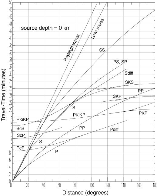
Figure 15. Standard travel time
curves for various seismic arrivals for a standard Earth model and a zero depth
of focus (from the
2.4 An additional example of the use of
EqLocate (a local event – the
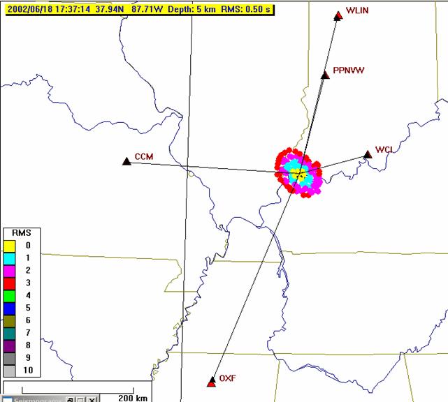
Figure 16. Stations (red triangles)
and trial epicenters (colored dots) for the
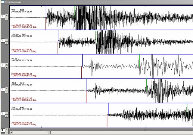
Figure 17. Seismograms,
interpreted arrival times (“picks”; downward red lines), theoretical arrival
times (calculated for the hypocenter shown in Figure 16; upward blue lines), a
calculated S-wave arrival times (upward green lines) for the southern
![]()
3. Importing
Data into EqLocate: Detailed
instructions for accessing data (SAC-format seismograms) from SpiNet (primarily
AS-1 seismograms) and from the IRIS DMC archive (GSN, PEPP and other
seismograms that can be downloaded in SAC format) using the WILBER II online
tool are provided at:
http://web.ics.purdue.edu/~braile/edumod/as1lessons/UsingAmaSeis/UsingAmaSeis.htm
(see section 5).
When adding data to EqLocate data folders use the WILBER II SAC binary, individual files option. Also, rename the seismogram files to use a short file name (similar to the file names used in this tutorial) so that many seismograms can be opened by the EqLocate Open command. PEPP and AS-1 records in SAC format can also be added.
Pre-assembled data sets for use in EqLocate are provided in section 4, below.
![]()
4. Data Sets: Some data sets (including some of those shown below) are included in the
download of EqLocate (from Alan Jones’ website). To download seismograms for the events shown
in Table 3, select the seismograms from the lists for the following events and
place the downloaded .sac files in folders (named for the events) in your
EqLocate folder.
Table
3. EqLocate earthquakes. Folders contain seismograms. Event is earthquake name. Origin time
(UTC/GMT), hypocenter and magnitude information in column to right (Yr = Year,
Mo = Month, Da = Day, Hr = Hour, Mn = Minutes, SS.ss = Seconds and decimal
seconds, Lat = Latitude in degrees [South is negative], Lon = Longitude in
degrees [West is negative], Dep = Depth of focus in kilometers, M = Magnitude).
|
Folder |
Event |
Yr Mo
Da HrMnSS.ss Lat
Lon Dep M |
|
1.
|
|
1994
06 09 003316.23 -13.84 -67.55
631 8.2 |
|
2. |
|
2000
04 23 092723.32 -28.31 -62.99 608 7.0 |
|
3. Cent. Amer. 1 |
|
1999
09 30 163115.69 16.06 -96.93 60 7.5 |
|
4. Pacific NW 1 |
|
2001
02 28 185432.83 47.15 -122.73
51 6.8 |
|
5. |
|
2002
04 20 105047.50 44.51 -73.70
11 5.2 |
|
6. W. Pacific 1 |
|
1995
01 16 204652.12 34.58 135.02
21 6.9 |
|
7. |
Northridge |
1994
01 17 123055.39 34.21 -118.54
18 6.8 |
|
8. |
So. |
2002
06 18 173715.20 37.99
-87.78 5 5.0 |
|
9. |
|
2001
04 21 171856.95 42.92 -111.39
0 5.4 |
|
10. |
Kodiak Is. Reg |
2001
01 10 160244.23 57.08 -153.21
33 7.0 |
- Folder/Event
= “S. America 1”: BOCO.BHZ.SAC,
NNA.BHZ.SAC,
SJG.BHZ.SAC,
LPAZ.BHZ.SAC,
RPN.BHZ.SAC.
- Folder/Event
= “S. America 2”: BDFB.BHZ.SAC,
NNA.BHZ.SAC,
SJG.BHZ.SAC,
PLCA.BHZ.SAC,
RCBR.BHZ.SAC.
- Folder/Event
= “Central America 1”: AMNO.LHZ.SAC,
COLA.LHZ.SAC,
KIP.LHZ.SAC,
BINY.LHZ.SAC,
HKT.BHZ.SAC;
for a relatively simple data set, try stations AMNO, COLA, KIP and BINY.
- Folder/Event
= “Pacific NW 1”: ADK.BHZ.SAC,
COR.BHZ.SAC,
FFC.BHZ.SAC,
KDAK.BHZ.SAC,
NEW.BHZ.SAC,
TUC.BHZ.SAC,
AMNO.BHZ.SAC,
DUG.BHZ.SAC,
INK.BHZ.SAC,
MA2.BHZ.SAC,
SFJ.BHZ.SAC;
for a relatively simple data set, try stations COR, FFC, KDAK, NEW, TUC
and AMNO.
- Folder/Event
= “Eastern US 1”: BINY.BHZ.SAC,
LBNH.BHZ.SAC,
NCB.BHZ.SAC,
HRV.BHZ.SAC,
MCWV.BHZ.SAC.
- Folder/Event
= “Western Pacific 1”: ARU.BHZ.SAC,
GUMO.BHZ.SAC,
MA2.BHZ.SAC,
TUC.BHZ.SAC,
YSS.BHZ.SAC,
FFC.BHZ.SAC,
NAI.BHZ.SAC,
NWAO.BHZ.SAC,
ULN.BHZ.SAC;
for a relatively simple data set, try stations GUMO, MA2, YSS and ULN.
- Folder/Event
= “California 1”: BAR.BHZ.SAC,
COR.BHZ.SAC,
NEE.BHZ.SAC,
PFO.BHZ.SAC,
TUC.BHZ.SAC,
CMB.BHZ.SAC,
ISA.BHZ.SAC,
PAS.BHZ.SAC,
SBC.BHZ.SAC,
VTV.BHZ.SAC;
for a relatively simple data set, try stations BAR, PFO, CMB, ISA, SBC and
VTV.
- Folder/Event
= “Central US 1”: ACSO.BHZ.SAC,
JFWS.BHZ.SAC,
MYNC.BHZ.SAC,
PPBNL.BHZ.SAC,
PPMUN.BHZ.SAC,
PPPCH.BHZ.SAC,
WLIN.AS1.SAC,
CCM.BHZ.SAC,
MCWV.BHZ.SAC,
OXF.BHZ.SAC,
PPEGH.BHZ.SAC,
PPNVW.BHZ.SAC,
SSPA.BHZ.SAC,
WMOK.BHZ.SAC,
GOGA.BHZ.SAC,
MIAR.BHZ.SAC,
PPBLO.BHZ.SAC,
PPFAY.BHZ.SAC,
PPPCC.BHZ.SAC,
WCI.BHZ.SAC;
for a relatively simple data set, try stations WLIN, CCM, OXF, PPNVW and
WCI.
- Folder/Event
= “Western US 1”: AMNO.BHZ.SAC,
COLA.BHZ.SAC,
NEW.BHZ.SAC,
CCM.BHZ.SAC,
COR.BHZ.SAC,
SSPA.BHZ.SAC,
CMB.BHZ.SAC,
DUG.BHZ.SAC;
for a relatively simple data set, try stations NEW, COR, CMB and DUG.
- Folder/Event
= “Alaska 1”: COLA.BHZ.SAC,
HKT.BHZ.SAC,
NEW.BHZ.SAC,
TLY.BHZ.SAC,
DUG.BHZ.SAC,
INK.BHZ.SAC,
RES.BHZ.SAC,
TUC.BHZ.SAC,
HIA.BHZ.SAC,
MDJ.BHZ.SAC,
SSE.BHZ.SAC;
for a relatively simple data set, try stations COLA, INK, RES, TUC and
MDJ.
Notes for additional
development of tutorial:
Add
Add intermediate
depth event to show minimum RMS error (larger errors for both shallower and
deeper hypocenters) ?
Questions
Teaching strategies
![]()
Bolt, B.A., Earthquakes and Geological Discovery,
Scientific American Library, W.H.
Herrmann, R.B., FASTHYPO: A hypocenter location program, Earthquake Notes, 50 (2), 25-37, 1979.
![]()
Alan Jones’ development of the EqLocate computer code was supported by
IRIS and the National Science Foundation.
John Lahr provided useful suggestions on the program and for this
tutorial.
[1]  Last
modified March 13, 2006
Last
modified March 13, 2006
The web page for this document is: http://web.ics.purdue.edu/~braile/edumod/eqlocate/tutorial.htm.
Funding for this development provided by IRIS and the National Science Foundation.
ã Copyright 2003-4. L. Braile. Permission granted for reproduction for non-commercial uses.